Table of Contents
This section presents how to build a simple classification tree model. Other types of models are built in a similar way.
The first thing to do is to decide what data we want to use to build the model. Make sure you have the default alias properly set before proceeding. To define alias use Services component and Alias dialog which are described in chapter AdvancedMiner Client Graphical User Interface in the Services section.
This example uses the 'iris' data set. First we have to build PhysicalData:
pd = PhysicalData('iris')and now we can create LogicalData:
ld = LogicalData(pd)
The above procedure can also be performed using the graphical interface:
Right-click on Repository added in the Projects window, choose New ->Physical Data as shown below:

A window with the list of all tables will appear, select the one you are interested in ('iris') and click 'Next'.

A window for providing the name of our physical data object will appear. Enter 'pd' and click 'Next'. The new Physical Data object with the selected name will appear in the Projects window. Logical data can be created in the same way by choosing the New ->Logical Data menu command. A window (part of it is shown below) with the available physical data sets will appear. Select the one you wish to use from the list and click 'Finish'.

The second thing we have to do is to decide what kind of model we want to build and create a suitable FunctionSettings object:
cfs = ClassificationFunctionSettings()
We need to assign a data set to the FunctionSettings object:
cfs.logicalData = ld
select the attribute that we want to use as the target:
cfs.getAttributeUsageSet().getAttribute('Class').setUsage(UsageOption.target)and decide which learning algorithm to use:
cfs.algorithmSettings = TreeSettings()
The FunctionSettings object can be also created by using the graphical interface: click right button on the repository in the Projects component. It will activate a context menu; then choose New ->Mining Function from the menu. Choose the settings from the list and then enter a name for the new Function Settings object.

The new object, which includes attributeUsageSet, will appear in the Projects window. Next we need to add to this object (using its context menu) the corresponding logicalData and algorithmSettings objects:

After choosing algorithmSettings a window with the list of all available settings will appear and you will be able to select a suitable one (TreeSettings):

In order to finish the creation of the FunctionSettings object it is necessary to open attributeUsageSet (by double-clicking or right-clicking and choosing Open from the context menu) and selecting one variable as the target:

Some other variables can be selected as obligatory, active, inactive, etc. Active means that the variable can be used as an independent variable in the model. A variable which is set to inactive will not be used in the model. Some models allow to force a variable to be used by setting the usage type to obligatory.
Now we need to build MiningBuildTask. First, however, it si necessary to save PhysicalData and FunctionSettings in the Metadata Repository. Until now all object were created locally. Objects have to be saved in the repository in order to be seen by AdvancedMiner Server. While creating MiningBuildTask we have to declare PhysicalData and FunctionSettings by names:
save('physical_data', pd)
save('cfs_Tree', cfs)
We can now build the task:
mbt = MiningBuildTask('physical_data', 'cfs_Tree', 'model_name' )We have to save MiningBuildTask to be able to execute it:
save('mbt_Tree', mbt)and finally we can execute this task:
execute('mbt_Tree')As the result we get a model called 'model_name'. See the figure below for what objects appear in the repository after executing the code above.

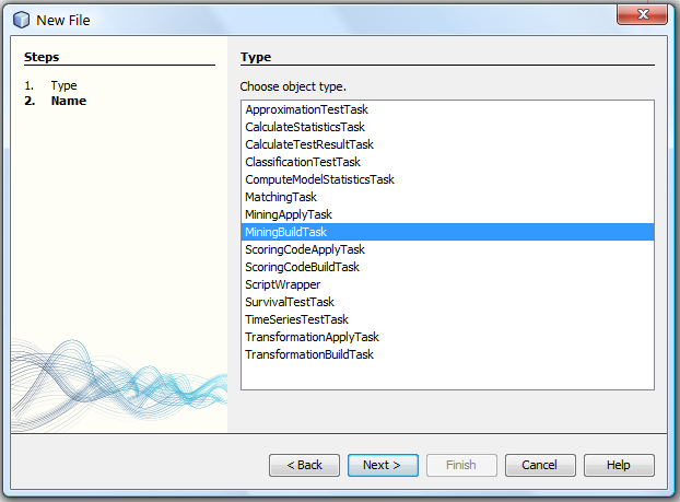
The procedure of model building can also be carried out using the graphical interface: choose the New ->Task item in the context menu and select the type of the task from the list:
Click 'Next', enter the name for the created task and click 'Finish'.
The next step is to add to the newly created MiningBuildTask all the required elements (functionSettings, buildData and model):

The model name reference is set by entering the model name in the creation wizard window and pressing 'Finish'.

After all the steps aboveare completed the created objects can be tested to see if no problems are found. Save them by pressing the 'Save' button on the main toolbar by choosing File -> Save from the menu.
To execute the created MiningBuildTask press F6 or right-click on the task object and choose 'Execute' from the context menu.
Note
The new model name is the same as the one set in MiningBuildTask, even if the model with the same name existed in the repository before the execution. In such case the following naming convention is used: The newest model is always named as in MiningBuildTask. The oldest model is named 'model_name_1', the second created model is named 'model_name_2' and so on. This rule guarantees that existing models do not change their names.
The first step of approximation model building is to load the data. Some approximation methods require a special data type or data preprocessing. All the necessary information about the proper preparation of data can be found in the Data requirements section of the chapter describing the appropriate method in the Modules part.
Note
For every approximation method the target attribute has to be numerical.
The second step is to select a classification method. The FunctionSettings object can be created as follows:
afs = ApproximationFunctionSettings()
If we test the created object the following message will appear:
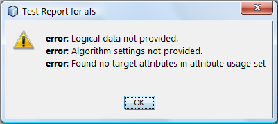
Logical data not provided
LogicalData should be assigned. It can be done by:
afs.logicalData = ld
where 'ld' denotes the LogicalData object created before.
Algorithm settings not provided
The choice of the method in AdvancedMiner is equivalent to the choice of the corresponding algorithm settings. In AdvancedMiner the following approximation methods are available: Linear Regression, Weighted Regression, IRLS, and Neural Networks.
Target attribute not specified
The target attribute should be specified. It can be done with
afs.targetAttributeName = 'Target_Attribute_Name'

The last step is the creation and execution of MiningBuidTask. It is described in the Model building section.
The first step of classification model building is to load the data. Some of the classification methods require a special data type or data preprocessing. All the necessary information about the proper data preparation can be found in the section Data requirements in the chapter describing the selected method in the Modules chapter.
Note
For every classification method the target attribute has to be categorical.
The second step is to select a classification method. FunctionSettings object can be created as follows:
cfs = ClassificationFunctionSettings()
If we test the created object the following message will appear:

Logical data not provided
LogicalData should be assigned. It can be done by:
cfs.logicalData = ld
where 'ld' denotes the LogicalData object created before.
Algorithm settings not provided
The choice of the method in AdvancedMiner is equivalent to the choice of the corresponding algorithm settings. In AdvancedMiner the following classification methods are available: Kohonen Maps, Neural Networks, Classification Trees, Logistic Regression, Bivariate Probit, Discriminant Analysis.
Table 15.2. Classification Methods - Algorithm Settings
Method Algorithm Settings Object Name Bivariate Probit BivariateProbitSettings
Discriminant Analysis DiscriminantSettings
Neural Networks FeedforwardNeuralNetSettings
Kohonen Maps KohonenClassificationSettings
Logistic Regression LogisticRegressionSettings
Classification Trees TreeSettings
Target attribute not specified
The target attribute should be specified. It can be done by:
cfs.targetAttributeName = 'Target_Attribute_Name'

The last step is the creation and execution of MiningBuidTask. It is described in the Model building section.
The first step of clustering model building is to load the data. All the necessary information about the proper data preparation can be found in the section Data requirements in the Kohonen Maps section.
The second step is to select a clustering method. A FunctionSettings object can be created as follows:
cfs = ClusteringFunctionSettings()
If we test the created object the following message will appear:
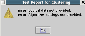
Logical data not provided
LogicalData should be assigned. It can be done by:
cfs.logicalData = ld
where 'ld' denotes the LogicalData object created before.
Algorithm settings not provided
The choice of the method in AdvancedMiner is equivalent to the choice of the corresponding algorithm settings. Kohonen Maps and KMeans are clustering methods available in AdvancedMiner. The algorithm settings can be provided by:
cfs.algorithmSettings = KohonenClusteringSettings()
The last step is the creation and execution of MiningBuidTask. It is described in the Model building section.
In order to build the Cox survival model it is necessary to create MiningBuildTask with the given data and Cox settings. Recall that the Cox model requires additional settings: censor and censoredValue:

The censor variable is set in functionSettings->attributeUsageSet and Censored category is set in the functionSettings.
Application of the built model will produce the output data which can be stored in a database or file. The output will contain the predicted survival time and the data used.