The data set for constructing a time series model should contain numerical target attribute (containing time series values) and an attribute containing time point identifier, used for time series values ordering. The name of the latter attribute has to be specified in time series function settings. In case of MGARCH(p,q) model, additional explanatory (i.e. active and obligatory) attributes (predictors) should also be numerical. In order to use categorical explanatory variables it is necessary to transform them into binary zero-one dummy variables.
Missing values are not supported by the Time Series Module unless Automatic Data Trasformation option is selected. The other way to use a data set with missing values is to replace the missing data before building the model or to switch to Liberal Mode in algorithm settings to automatically omit observations containing missing values.
Model building is performed in a standard way and the complete procedure is described in the chapter AdvancedMiner in Practice. The dedicated Function Settings for time series analysis are TimeSeriesFunctionSettings. After adding LogicalData we add AlgorithmSettings. Two types of AlgorithmSettings are available: ARCHSettings and GARCHSettings depending on what type of model is desired. Next, at the TimeSeriesFuctionSettings Properties window we set 2 basic properties: Target - the name of dependent variable and the Time Point Attribute Name - the name for variable indicating time points. The option Sorting Required - specifies whether sorting by time variable is needed.
Full specification of the model settings contains the elements of the Algorithm Settings: General Algorithm Settings, Optimization Algorithm Settings and Variable Selection Settings and Transformation Settings.
Table 41.1. Time Series: General Algorithm Settings
| Name | Description | Possible values | Default value |
|---|---|---|---|
| Autocorrelation Test Span | the number of timepoints used for creation of sample autocorrelation and partial autocorrelation plots | Positive integer numbers | 10 |
| P | p parameter of GARCH(p,q) model | Positive integer numbers | 1 |
| Q | q parameter of ARCH(q) and GARCH(p,q) models | Positive integer numbers | 1 |
| Automatic Data Transformations | if TRUE automatic transformations (e.g. replaceMissing, binarization) should be executed, false otherwise. | TRUE / FALSE | FALSE |
| Confidence Level | the confidence level value for the calculation of interval estimators for model parameters | Real numbers from interval (0,1) | 0.95 |
| Execute Init Tests | if TRUE initial data/task tests should be executed, false otherwise | TRUE / FALSE | TRUE |
| Group Statistics | if TRUE statistics for variable groups should be computed, false otherwise | TRUE / FALSE | FALSE |
| Intercept | TRUE / FALSE | TRUE | |
| Liberal Execution Mode | if TRUE 'liberal' execution is preferred (do not stop on minor errors), false otherwise | TRUE / FALSE | TRUE |
| Preselection | True if univariate p-value statistics should be computed | TRUE / FALSE | FALSE |
In addition to the settings specific to the Bivariate Probit algorithm, the user can use:
Variable Selection Settings - to control the behavior of the available heuristics for model building; these settings are described in the Automatic Variable Selection chapter
Optimization Algorithm Settings - to control the selection of the optimization algorithm; these settings are described in the Optimization Library chapter.
Transformation Settings - to control the way of data transformation; these settings are described in the Transformation chapter.
Table 41.2. Time Series Model Statistics: Variables Statistics
| Name | Description |
|---|---|
| Coeff | the value of the estimated parameter |
| Univariate Pr>ChiSq | the p-value for the residual Likelihood Ratio statistic calculated for the univariate model. This statistic is calculated only if the Preselection option has been selected in the current algorithm settings |
| Lower Confidence | the lower bound of the confidence interval for the current estimator. The confidence interval is calculated for confidence level specified in the current algorithm settings (see the Confidence Level option) |
| Upper Confidence | the upper bound of the confidence interval for the current estimator. The confidence interval is calculated for confidence level specified in the current algorithm settings (see the Confidence Level option) |
| StdErr | the standard error of the parameter estimator |
| Wald Test | the Wald statistic for the parameter estimator |
| Pr(Wald>ChiSq) | the p-value for the Wald statistic for parameter estimator. The statistic is tested with the chi-square distribution with one degree of freedom |
Table 41.3. Time Series Model Statistics: Model Statistics
| Name | Description |
|---|---|
| Likelihood Ratio Stat | the value of the Likelihood Ratio statistic |
| Pr(LRatio>ChiSq) | the p-value for the Likelihood Ratio statistic. The statistic is tested with the chi-square distribution with p degrees of freedom (where p is the number of attributes included in the final model) |
| Score Stat | the value of the Score statistic |
| Pr(Score>ChiSq) | the p-value for the Score statistic The statistic is tested with the chi-square distribution with p degrees of freedom (where p is a number of attributes included in the final model) |
| Wald Stat | the value of the Wald statistic |
| Pr(Wald>ChiSq) | the p-value for the Wald statistic. The statistic is tested with the chi-square distribution with p degrees of freedom( where p is a number of attributes included in the final model) |
Model Testing for Time Series is an experimental feature.
TimeSeries test task is to some extent analogous to approximation testing process. I.e. test aims at calculation of some aggregated statistics on how good variance predicted from the model approximate observed series variance. Available statistics include:
MeanAbsoluteError (MAE) -

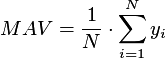
MeanActualValue (MAV) - observed mean of the whole serie:
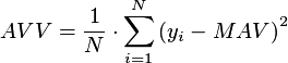
ActualValueVariance (AVV) - observed variance of the whole series:
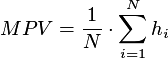
MeanPredictedVariance (MPV) - mean value of the predicted variances:
RMSError -

RSquaredError -
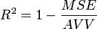
where  is the current mean value of the series,
 denotes model variance for i-th observation,
 denotes the series value for i-th observation ang N means the number of observations
of the series.
denotes the series value for i-th observation ang N means the number of observations
of the series.
Model Applying for Time Series is an experimental feature.
Application of ARCH(p) or GARCH(p,q) time series models is aimed at estimation of the forecasted value of series variance at time point t+1. At the moment, only one-step-ahead forecasting mode is available.
For details on how to apply the model to the data see the chapter Applying Models in AdvancedMiner subsection Applying for different mining functions section.
After time series model application, output table contain following columns:
Table 41.4. Time Series - Apply output columns
| output column | description | |
| <prefix>_<timepoint> attributes | model-forecasted values of the variance for timepoints t + 1, t + 2, etc. where t is timepoint for the current observation; prefix can be set using setPrefix method in TimeSeriesApplyOutput (default prefix is “variance”) | |
| regressed_mean | containing linear score
 calculated from the linear part of the GARCH model; in case when no
explanatory attribute is present in the model, regressed mean reduces
to intercept value
calculated from the linear part of the GARCH model; in case when no
explanatory attribute is present in the model, regressed mean reduces
to intercept value
| |
| forecast_lowerbound | lower bound of the confidence interval for the forecasted variance at t + 1; confidence intervals are calculated for 95% confidence level | |
| forecast_upperbound | upper bound of the confidence interval for the forecasted variance at t + 1; confidence intervals are calculated for 95% confidence level |