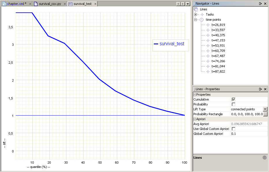
The Survival module can be used to predict the distribution of survival time for individuals in a given population, to investigate the strength of the influence of particular variables on the expected survival time and to compare survival time distributions among different subpopulations.
The data set for any survival analysis application should contain a categorical binary censor attribute and a numerical target attribute.
Additionally, the data for the semi-parametric Cox model estimation should contain numerical explanatory (active/obligatory) attributes. In order to use categorical explanatory variables it is necessary to convert them to binary zero-one dummy variable using the binarize procedure with the Random Redundant option switched on or to use Automatic Data Transformation option.
Missing values are not supported by Survival Analysis module unless Automatic Variable Transformations options is on. The other way to use a data set with missing values is to apply the ReplaceMissing transformation before building the model.
Model building and testing is performed in the standard way and the complete procedure is described in the chapter AdvancedMiner in Practice (see Survival).
The nonparametric survival model is controlled by the following algorithm settings:
Table 39.1. Survival Module: Algorithm Settings
There is no special model statistics for non-parametric survival models. The estimated values, standard errors and confidence intervals of the empirical survival (S0), empirical cumulated hazard (H0), empirical hazard (h0) and probability density functions (pdf) are available in AdvancedMiner Script. An example script can be found in the Appendix Examples. The non-parametric model contains also the plots of the empirical hazard and empirical survival functions, together with the lower and upper confidence intervals for the respective functions.
Full specification of the Cox model settings contains the elements of the Algorithm Settings: General Algorithm Settings, Optimization Algorithm Settings and Variable Selection Settings and Transformation Settings.
The Cox algorithm is controlled by the following options:
Table 39.2. Survival Module: Algorithm Settings
| Name | Description | Possible values | Default value |
|---|---|---|---|
| Automatic Data Transformations | if TRUE automatic transformations (e.g. replaceMissing, binarization) should be executed, false otherwise. | TRUE / FALSE | FALSE |
| Confidence Level | the value of the confidence level for the calculation of interval estimators for model parameters | real numbers from the interval (0.5,1) | 0.95 |
| Execute Init Tests | if TRUE initial data/task tests should be executed, false otherwise | TRUE / FALSE | TRUE |
| Group Statistics | if TRUE statistics for variable groups should be computed, false otherwise | TRUE / FALSE | FALSE |
| Liberal Execution Mode | if TRUE 'liberal' execution is preferred (do not stop on minor errors), false otherwise | TRUE / FALSE | TRUE |
| Preselection | a binary switch for the calculation of the p-value statistic for univariate models | TRUE / FALSE | FALSE |
| Tie Handling Method | which method to use for handling tied observations (currently only the Breslow method is available) | breslow | breslow |
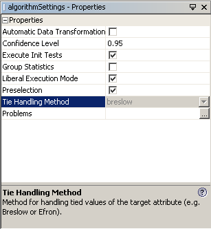
In addition to the settings specific to the Survival algorithm, the user can use:
Variable Selection Settings - to control the behavior of the available heuristics for model building; these settings are described in the Automatic Variable Selection chapter
Optimization Algorithm Settings - to control the selection of the optimization algorithm; these settings are described in the Optimization Library chapter.
Transformation Settings - to control the way of data transformation; these settings are described in the Transformation chapter.
Note
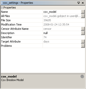
In order to build the Cox model it is necessary to choose Censor (the name of censored variable) and Censored Category (the censor value for the censored observation) in the survival function settings. For more details see the chapter Practice.
The final semi-parametric Cox model contains the following statistics: Variable Statistics, Model Statistics, Correlation and Covariance matrices.
Table 39.3. Survival Model Statistics: Variables Statistics
| Name | Description |
|---|---|
| Univariate Pr>ChiSq | the p-value for the residual Likelihood Ratio statistic calculated for the univariate model. This statistic is calculated only if the Preselection option has been selected in the current algorithm settings |
| Coeff | the value of the estimated parameter |
| Lower Confidence | the lower bound of the confidence interval for the current estimator. The confidence interval is calculated for confidence level specified in the current algorithm settings (see the Confidence Level option) |
| Pr(Wald>ChiSq) | the p-value for the Wald statistic for parameter estimator. The statistic is tested with the chi-square distribution with one degree of freedom |
| Scaled Schoenfeld residual mean | the mean value of the Scaled Shoenfeld Residuals |
| Schoenfeld residual mean | the mean value of the Shoenfeld Residuals |
| StdErr | the standard error of the parameter estimator |
| Upper Confidence | the upper bound of the confidence interval for the current estimator. The confidence interval is calculated for confidence level specified in the current algorithm settings (see the Confidence Level option) |
| Variable | attribute name |
| Wald Test | the Wald statistic for the parameter estimator |
- Scaled Shoenfeld Residuals
Scaled Shoenfeld Residuals are calculated for each observation as approximation using the fact that the covariance matrix of the vector of residuals tends to be fairly constant over time (see Grambsch and Therneau 1994):

Here
 is a vector of
Shoenfeld residuals for each observation and
is a vector of
Shoenfeld residuals for each observation and  is the observed number of
uncensored survival times.
is the observed number of
uncensored survival times.- Shoenfeld Residuals
Schoenfeld Residuals are calculated for each variable as:
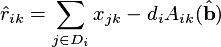
where
 are defined in the Partial likelihood
function section (for details see Schoenfeld 1982).
are defined in the Partial likelihood
function section (for details see Schoenfeld 1982).- Wald statistic
The Wald statistic for parameter estimator is
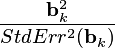

where H stands for the Hessian matrix (the matrix of the second order partial derivatives of the log-likelihood function) and U is the gradient (the vector of the first order partial derivatives of the log-likelihood function), both calculated for the maximum likelihood estimator (MLE).
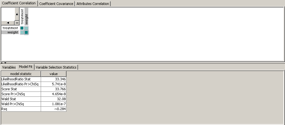
Table 39.4. Survival Model Statistics: Model Statistics
| Name | Description |
|---|---|
| Likelihood Ratio Stat | the value of the Likelihood Ratio statistic |
| Pr(LRatio>ChiSq) | the p-value for the Likelihood Ratio statistic. The statistic is tested with the chi-square distribution with p degrees of freedom (where p is the number of attributes included in the final model) |
| Pr(Score>ChiSq) | the p-value for the Score statistic The statistic is tested with the chi-square distribution with p degrees of freedom (where p is a number of attributes included in the final model) |
| Pr(Wald>ChiSq) | the p-value for the Wald statistic. The statistic is tested with the chi-square distribution with p degrees of freedom( where p is a number of attributes included in the final model) |
| Rsq | the  statistic statistic |
| Score Stat | the value of the Score statistic |
| Wald Stat | the value of the Wald statistic |
- Likelihood Ratio statistic
The Likelihood Ratio statistic is calculated as:


The
 statistic is defined
as:
statistic is defined
as:
where N is the total number of observations.
- Score statistic
The Score statistic is defined as:

where
 is the gradient
of the log-likelihood function.
is the gradient
of the log-likelihood function.- Wald statistic
The Wald statistic is defined as:

where H stands for the Hessian matrix (the matrix of the second order partial derivatives of the log-likelihood function) and U is the gradient (the vector of the first order partial derivatives of the log-likelihood function), both calculated for the maximum likelihood estimator (MLE).
Table 39.5. Survival Model Statistics: Covariance
| Name | Description |
|---|---|
| Covariance | the covariance matrix of the parameter estimators |

 is the Hessian matrix of the
parameters estimators.
is the Hessian matrix of the
parameters estimators.Table 39.6. Survival Model Statistics: Correlation
| Name | Description |
|---|---|
| Correlation | the correlation matrix of the parameters estimators |

 are the
 -th elements of the covariance
matrix of the parameter estimators.
-th elements of the covariance
matrix of the parameter estimators.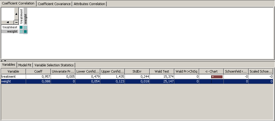
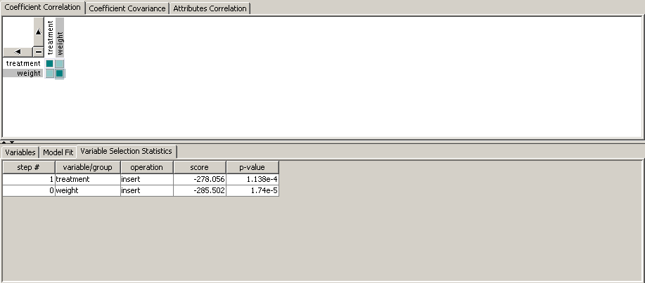
If any of the automatic variable selection methods was chosen during model building (i.e. Variable Selection Method option was set to forward, backward or stepwise) then the final model statistics, beside previously mentioned elements, also contain the history of variable selection steps. Each entry corresponds to one step and consists of the name of the inserted/removed variable and the p-value for the residual Likelihood Ratio test.
Non-parametric survival models cannot be applied nor tested.
In order to apply the Cox model it is necessary to create a MiningApplyTask with the given data and settings (see the chapter Practice). Recall that the Cox model building and testing require additional settings: Censor and Censored Category:
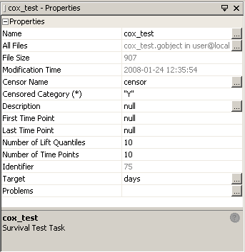
Applications of the survival model is done in much the same way as described in the Applying Models in AdvancedMiner. The major difference is in the specialized SurvivalApplyOutput which we choose while adding applyOutput the MiningApplyTask. Next, we set properties of the applyOutput: prefix - which is the name of prefix used to create output column names, first/last time point which describe bounds of the time scale interval and number of time points which describe the number of successive points in time.
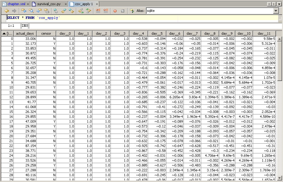
Application of the built model will produce output data which can be stored in a database or a file. The output will contain the predicted survival time and the data used.
Below are examples of output windows: