The data set for constructing a logistic regression model should contain numerical explanatory (i.e. active and obligatory) attributes and a binary target attribute. In order to use categorical explanatory variables it is necessary to transform them into binary zero-one dummy variables. Binarization can be performed before building the model or during building process by selecting Automatic Data Trasformation option in General Algorithm Settings.
Missing values are not supported by the Logistic Regression Module unless Automatic Data Trasformation option in General Algorithm Settings is selected. The other way to use a data set with missing values is to replace the missing data before building the model or to switch to Liberal Mode in algorithm settings to automatically omit observations containing missing values.
Model building and testing is performed in a standard way and the complete procedure is described in the chapter AdvancedMiner in Practice (see Classification). Full specification of the model settings contains the elements of General Algorithm Settings, Optimization Algorithm Settings, Variable Selection Settings and Transformation Settings.
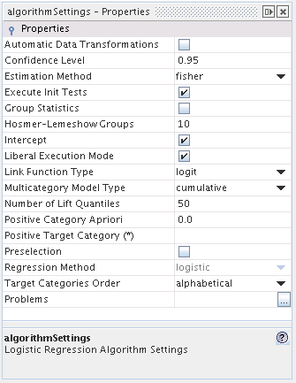
Logistic Regression has the following algorithm and function settings:
Table 38.1. Logistic Regression: General Algorithm Settings
| Name | Description | Possible values | Default value |
|---|---|---|---|
| Automatic Data Transformations | if TRUE automatic transformations (e.g. replaceMissing, binarization) should be executed, false otherwise. | TRUE / FALSE | FALSE |
| Confidence Level | the confidence level value for the calculation of interval estimators for model parameters | real numbers from the interval (0.5,1) | 0.95 |
| Estimation Method | sets the estimation algorithm for the logistic regression model | fisher / newton | fisher |
| Execute Init Tests | if TRUE initial data/task tests should be executed, false otherwise | TRUE / FALSE | TRUE |
| Group Statistics | if TRUE statistics for variable groups should be computed, false otherwise | TRUE / FALSE | TRUE |
| Hosmer-Lemeshow Groups | the number of groups of observations used in the Hosmer-Lemeshow statistic. The observations ordered according to increasing probability of positive response are divided into g groups | positive integer numbers | 10 |
| Intercept | selects the model type: regression model with intercept if TRUE and without intercept if FALSE | TRUE / FALSE | TRUE |
| Liberal Execution Mode | if TRUE 'liberal' execution is preferred (do not stop on minor errors), false otherwise | TRUE / FALSE | TRUE |
| Link Function Type | sets the type of the probability link function | logit / probit | logit |
| Multicategory Model Type | Multicategory model type | binary / cumulative / multinomial | binary |
| Number of Lift Quantiles | The number of quantiles for lift computation | Positive integer value | 50 |
| Positive Category Apriori | the a priori probability of the occurrence of a positive category | real numbers from the interval (0,1) | - |
| Positive Target Category | positive (event) category value for the target attribute | attribute name | - |
| Preselection | if preselection is set to TRUE then the Univariate Pr>ChiSq statistic is calculated for each variable included in the model | TRUE/ FALSE | FALSE |
| Target Categories Order | sets the order of the categories of the target attribute | dataOrder / alphabetical / alphabeticalDesc | alphabetical |
- Model Estimation Method
The option newton sets the Newton-Raphson algorithm as the method for finding the maximum of the likelihood function. The Hessian (the matrix of partial derivatives of the second order), which is used in the Newton-Raphson algorithm is approximated by the BHHH estimator (see Berndt et al. (1974)).
The vector of model parameters
 is
estimated by the maximization of the logarithm of the likelihood
function (the notation is introduced in the Method Description
section):
is
estimated by the maximization of the logarithm of the likelihood
function (the notation is introduced in the Method Description
section):
Finding this maximum is equivalent to finding the critical points of the likelihood function, i.e. to solving a system of n (or n+1 if INTERCEPT = TRUE) equations
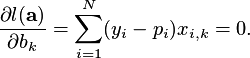
The option fisher sets the Fisher scoring algorithm (compare with the Lawless Singhal algorithm in Hosmer and Lemeshow (1989) page 129) as the method for estimating model parameters using the iterative formula:


where X is the matrix of observations,


Note
Presented forms of the Z and W are correct only for logit link function.- Link Function Type
The option logit sets the logit link function, i.e. the model will have the following form:

The option probit sets the probit link function, i.e. the model will have the following form:

where
 is the
cumulative distribution function of the standard normal
distribution.
is the
cumulative distribution function of the standard normal
distribution.- Positive Category Apriori, Positive Target Category
Specifies the true a priori probability for the positive category (selected by setting the Positive Target Category) occurrence in the given population. This option is useful for choice-based samples, when the positive category frequency in build data differs from a-priori probability. If Positive Category Apriori is not set, the proportion from the sample is taken. If Positive Target Category is not set, the first category in the specified order will be the default positive category.
- Target Categories Order
Specifies the order, in which target categories will appear in the model. The default value is alphabetical, which means appearance in the order of ascending numerical values or alphabetical categorical values. The value alphabeticalDesc means descending order. The value dataOrder means the order in which categories appear in the input data table.
In addition to the settings specific to the Logistic Regression algorithm, the user can use:
Variable Selection Settings - to control the behavior of the available heuristics for model building; these settings are described in the Automatic Variable Selection chapter
Optimization Algorithm Settings - to control the selection of the optimization algorithm; these settings are described in the Optimization Library chapter
Transformation Settings - to control the way of data transformation; these settings are described in the Transformation chapter.
The final model contains the following statistics: Variable Statistics, Group Statistics (only if Group Statistics is set), Model Fit Statistics, Variable Selection Statistics (only if Variable Selection Method is forward, backward or stepwise), Coefficient Correlation and Covariance Matrices, Attributes Correlation Matrix and Auxiliary Lifts (only if VariableSelectionsSettings are properly set).
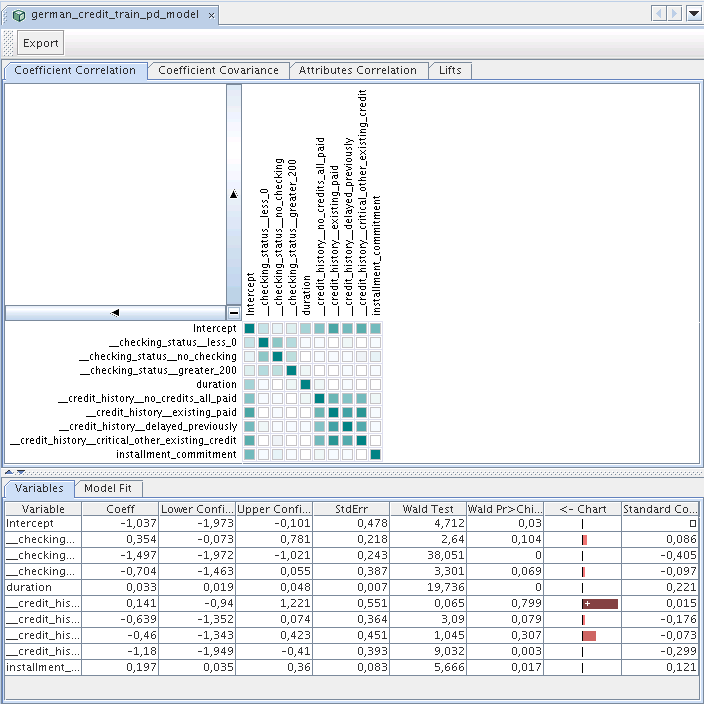
Table 38.2. Logistic Regression Model Statistics: Variables Statistics
| Name | Description |
|---|---|
| Variable | the attribute name |
| Univariate Pr>ChiSq | the p-value of the Likelihood Ratio statistic for the model containing only the variable (and optionally the intercept). This statistic is calculated only if preselection = TRUE |
| Coeff | the estimated coefficients values |
| Lower Confidence | the lower bound of the confidence interval for the current estimator. Te confidence interval is calculated for Confidence Level specified in the current algorithm settings. |
| Upper Confidence | the upper bound of the confidence interval for the current estimator. The confidence interval is calculated for the Confidence Level specified in the current algorithm settings. |
| StdErr | the standard error of the parameter estimator |
| Standard Coeff | the standardized coefficient values |
| Wald Test | the value of the Wald statistic for the variable (or attribute) |
| Wald Pr>ChiSq | the p-value of the Wald statistic for the attribute |
- Standard Coeff
The value of the Standard Coefficient of the variable (or attribute)
 is equal to:
where s_k is the total sample standard deviation for the k-th explanatory variable and

.
- Wald Test
The value of the Wald statistics the variable (or attribute)
 is equal to: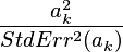
where
 and H is the
Hessian of the likelihood function evaluated at the point
and H is the
Hessian of the likelihood function evaluated at the point

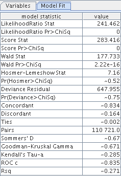
Table 38.3. Logistic Regression Model Statistics: Model Fit Statistics
| Name | Description |
|---|---|
| Concordant | the percentage of pairs of observations for which the model-estimated probability of an observation with a positive response is greater than the probability of an observation with a negative response |
| Deviance Pr>ChiSq | p-value of the Deviance statistics. The statistic is tested with the chi-square distribution with M-m degrees of freedom (M - the number of different subgroups of observations in the data, m - the number of attributes in the model (including intercept)). |
| Deviance Residual | the value of the Deviance statistic |
| Discordant | the percentage of pairs of observations for which the model-estimated probability of an observation with a positive response is smaller than the probability of an observation with a negative response |
| Goodman-Kruskal Gamma | the value of the Goodman-Kruskal Gamma statistic |
| Hosmer-Lemeshow Stat | the value of the Hosmer-Lemeshow statistic |
| Kendall's Tau-a | the value of Kendall's Tau-a statistic |
| LikelihoodRatio Stat | the value of the Likelihood Ratio statistic |
| Hosmer Pr>ChiSq | the p-value of the Hosmer-Lemeshow statistic. The statistic is tested with the chi-square distribution with degrees of freedom equal to the number of Hosmer-Lemeshow Groups. |
| LRatio Pr>ChiSq | the p-value of the Likelihood Ratio statistic. The statistic is tested with the chi-square distribution with m degrees of freedom (m is the number of attributes (variables) in the model). |
| Pairs | the number of data observations with a positive response multiplied by the number of observations with a negative response. It may be interpreted as the number of pairs of observations such that one observation has a positive and the other has a negative response |
| ROC c | the value of the ROC c statistic |
| Rsq | the value of the  statistic
 |
| Score Pr>ChiSq | the p-value of the score statistic. The statistic is tested with the chi-square distribution with m degrees of freedom(m is the number of attributes (variables) in the model). |
| Score Stat | the value of the score statistic (for more details see Cox and Hinkley 1974, Section 9.3) |
| Sommers' D | the difference between the Concordant and the Discordant |
| Ties | the percentage of pairs of observations for which the model-estimated probabilities of observation with a positive response and of observation with a negative response are equal |
| Wald Pr>ChiSq | the p-value of the Wald statistic |
| Wald Stat | the value of the Wald statistic |
- Concordant
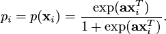
the percentage of pairs of observations for which the model-estimated probability of an observation with a positive response is greater than the probability of an observation with a negative response. The probabilities are calculated using the following formula:
- Deviance Statistic
The value of the deviance statistic, measuring the goodness of fit of the model, is calculated using the following formula:

And
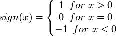
In the case when the observations are divided into M groups the formula for
 is more complex (see also
Hosmer and Lemeshow 1989,
p.146).
is more complex (see also
Hosmer and Lemeshow 1989,
p.146).- Goodman-Kruskal Gamma
This statistic is defined as:

where
 is the Concordant, and
 is the Discordant.
- Hosmer-Lemeshow Statistic
This statistic, measuring the goodness of fit of the model, is calculated using the formula:
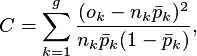
where
 denotes the number of test groups
(see the option Hosmer-Lemeshow
Groups),
denotes the number of test groups
(see the option Hosmer-Lemeshow
Groups),  is the number of observations in
the k-th group,
is the number of observations in
the k-th group,  denotes the number of observations
in the k-th group with a positive response (i.e. observations
for which the event, whose probability of occurrence we want to
predict, has occurred) and
denotes the number of observations
in the k-th group with a positive response (i.e. observations
for which the event, whose probability of occurrence we want to
predict, has occurred) and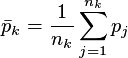
denotes the average predicted probability for the k-th group.
- Kendall's Tau-a
This statistic is defined as:
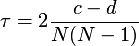
where
 stands for the number of Concordant pairs,
 stands for the number of Discordant
pairs and N is the number of observations.
stands for the number of Discordant
pairs and N is the number of observations.- LikelihoodRatio Stat
The Likelihood Ratio statistic is defined as:

If the indicator variables
 are binary (zero-one)
then the likelihood of the saturated model is equal to 1 and the
equation above can be simplified.
are binary (zero-one)
then the likelihood of the saturated model is equal to 1 and the
equation above can be simplified.- Wald P>ChiSq
This is the p-value of the Wald statistic for the attribute. If the attribute is not significant the statistic has approximately the chi-square distribution with one degree of freedom.
- ROC c
The area of the region under the plot of the Receiver Operating Characteristic (ROC) function is equal to:

where
 stands for the Concordant and
 stands for the Discordant.
This statistic is defined as:
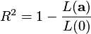
where

and L(0) denote the likelihoods of the estimated model and the model containing only the intercept, respectively.
- Wald Stat
The value of the Wald statistics is calculated as:

where H(a) stands for the Hessian of the likelihood function evaluated at the point
 .
.
Table 38.4. Logistic Regression Model Statistics: Group Statistics
| Name | Description | |
|---|---|---|
| Variable | the attribute name | |
| DF | number of degrees of freedom of variable or group of variables; in the second case numer of degrees is equal to the nuber of estimated parameters that means number of variables in group | |
| Wald Stat | the value of the Wald statistic | |
| Wald Pr>F | the p-value of the Wald statistic | |
| Univariate Pr>F | the p-value of the Likelihood Ratio statistic for the model containing only the variable (or group of variables) (and optionally the intercept). This statistic is calculated only if preselection = TRUE |
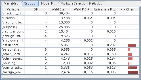
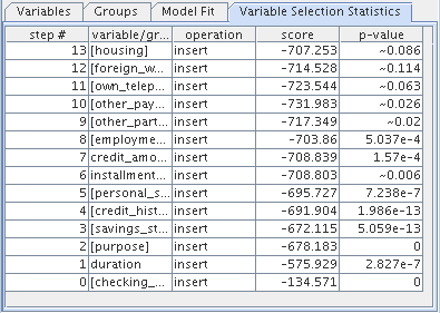
Table 38.5. Logistic Regression Model Statistics: Variable Selection Statistics
| Name | Description | |
|---|---|---|
| #step | iteration of variable selection algorithm | |
| variable/group | the attribute (group of attributes) name | |
| operation | action taken (remove / insert) due to variable during automatic variable selection process | |
| score | value for the model-dependent Residual Statistic | |
| p-value | the p-value for the model-dependent Residual Statistic |
In case of best subset variable selection algorithm the Variable Selection Statistics look differently.
Table 38.6. Logistic Regression Model Statistics: Variable Selection Statistics: best subset
| Name | Description | |
|---|---|---|
| # | iteration of variable selection algorithm | |
| model | best model from models of the size | |
| size | size of the model | |
| score | the value of the model-dependent Scoring Statistic |
Additionally, the covariance and correlation matrices of the coefficient estimators as well as the correlation matrix of the attributes are calculated and displayed:
Table 38.7. Logistic Regression Model Statistics: Coefficient / Attributes Correlation
| Name | Description |
|---|---|
| Coefficient/Attributes Correlation | the correlation matrix of the parameter estimators / attributes |
- Correlation
The correlation matrix for coefficient estimators is calculated as

where
 are the
 -th elements of the covariance matrix
of the parameter estimators.
-th elements of the covariance matrix
of the parameter estimators.Correlation between attributes is calculated in standard way.
Table 38.8. Logistic Regression Model Statistics: Coefficient Covariance
| Name | Description |
|---|---|
| Covariance | the covariance matrix of the parameter estimators |

 is the Hessian matrix of the
parameter estimators.
is the Hessian matrix of the
parameter estimators.- Lifts for main and transitional models
There are two base lifts, first is calculated for train data (always calculated), and the second one is calculated for validation data (if validation data is determined for build task). Except these two base lifts there are also auxiliary lifts which are calculated for transitional models. Transitional model is derived from the main model, and is built by removing one of variables. Auxiliary lifts can be determined respectively for train and validation data.
The auxiliary lifts are accessible in two places: in modelStatistics, where each lift can be visualized separately, and in the Lifts tab, where the lifts for the training data set and validating data set (if used) are displayed on the same chart. By clicking on the selected model variables (or group of variables- dependent on Group Mode setting in Variable Selection Settings) the user can display the appropriate auxiliary lifts on the chart. This provides the means for straightforward comparison of the main and transitional models.
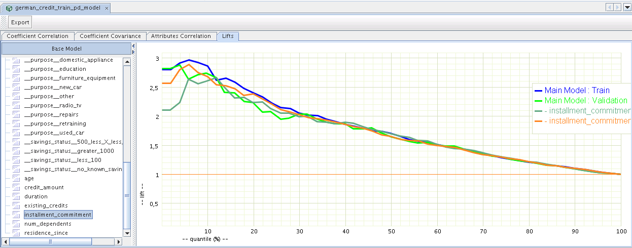
User can customize (turn on/off) auxiliary lifts by setting proper values in VariableSelectionSettings: Auxiliary Lift Estimation Mode and Auxiliary Statistics Mode.
Logistic Regression Module may be applied to classification problems. Classification is based on the estimated probabilities and is achieved by setting the threshold probability. A record (vector of attributes) is classified as belonging to one of the two groups based on the comparison between the conditional probability estimated for this record and the threshold probability (see also the example script below).
The Logistic Regression module is capable of creating several output types when classifying the provided data. For details on how to apply the model to the data see the chapter Applying Models in AdvancedMiner, and the Classification subsection in the Applying for different mining functions section.
The table below presents the possible combinations and descriptions of the output items and output types.
To explain statistics below we need some notation.
Let  be the scored probability
 for observation
  ,
where F is a link function.
,
where F is a link function.
Let  ,
where Cov(a) is the covariance matrix of the estimator.
,
where Cov(a) is the covariance matrix of the estimator.
Let  .
.
Table 38.9. Classification - Output items and output types combinations
| output type | output item type | description |
| probability | rank | returns the probability of the n-th best category |
| probability | category | returns the probability of classifying as given category |
| predictedCategory | rank | returns the n-th best category |
| predictedCategory | category | not supported |
| nodeId | rank | returns the structure id to which the input case was assigned. It depends on the particular algorithm what the term "structure" means. Some algorithms do not support this feature at all. Refer to the chapter describing the algorithm/module for more details. |
| nodeId | category | not supported |
| leverage | logistic regression |  |
| pearsonResidual | logistic regression |  |
| devianceResidual | logistic regression |  |
| dfbetas | logistic regression |  ,
where
,
where  is v-th element of the vector and
 is the v-th diagonal element of the matrix.
|
| c | logistic regression |  |
| cBar | logistic regression |  |
| deltaDev | logistic regression |  |
| deltaChiSq | logistic regression | 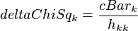 |
Note
In case of all the influence diagnostics it is required to have the target attribute in scored data. Moreover the target attribute name must be the same as in the build data.