The linear regression module can be used for data approximation.
The linear regression, weighted regression and IRLS regression models require numerical attributes. In order to use categorical explanatory variables it is necessary to transform them into binary zero-one dummy variables. Binarization can be performed before building the model or during building process by selecting Automatic Data Trasformation option in General Algorithm Settings .
Missing values are not supported by any model in the Linear Regression module unless Automatic Data Trasformation option in General Algorithm Settings is selected. The other way to use a data set with missing values is to replace the missing data before building the model or to switch to Liberal Mode in algorithm settings to automatically omit observations containing missing values.
Model building and testing is performed in the standard way and the complete procedure is described in the chapter AdvancedMiner in Practice (see Aproximation). Full specification of the model settings contains the elements of General Algorithm Settings, Optimization Algorithm Settings, Variable Selection Settings and Transformation Settings.
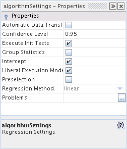
Linear regression modeling is controlled by the following algorithm settings:
Table 37.1. Linear, Weighted and IRLS Regression: General Algorithm Settings
| Name | Description | Possible Values | Default value |
|---|---|---|---|
| Automatic Data Transformations | if TRUE automatic transformations (e.g. replaceMissing, binarization) should be executed, false otherwise. | TRUE / FALSE | FALSE |
| Confidence Level | the confidence level value for the calculation of interval estimators for model parameters | real numbers from the interval (0.5,1) | 0.95 |
| Execute Init Tests | if TRUE initial data/task tests should be executed, false otherwise | TRUE / FALSE | TRUE |
| Group Statistics | if TRUE statistics for variable groups should be computed, false otherwise | TRUE / FALSE | TRUE |
| Intercept | determines the type of the model: linear regression with a constant term if TRUE and without a constant term if FALSE | TRUE / FALSE | TRUE |
| Liberal Execution Mode | if TRUE 'liberal' execution is preferred (do not stop on minor errors), false otherwise | TRUE / FALSE | TRUE |
| Preselection | whether to calculate the p-value statistic for univariate models | TRUE / FALSE | FALSE |
Univariate Model. This is a model consisting only of an intercept (if Intercept option is set to TRUE), a single explanatory variable and a dependent variable (target).
There are some additional algorithm settings for WLS and IRLS regression models.
Table 37.2. IRLS and Weighted Regression: additional Algorithm Settings
| Name | Description | Possible values | Default value |
|---|---|---|---|
| Weight Tuning Constant | the constant used in weight functions | any real number greater than 0.001 | 1.345 |
| Weight Type | the function used to compute the weights in each iteration | student/huber | huber |
IRLS Regression has also specific settings to control the non-linear optimization algorithm: Optimization Algorithm Settings .
In addition to the settings specific to the regression algorithms, the user can use:
Variable Selection Settings - to control the behavior of the available heuristics for model building; these settings are described in the Automatic Variable Selection chapter
Transformation Settings - to control the way of data transformation; these settings are described in the Transformation chapter.
The results of model building are reported in a modelStatistics object. The final model contains the following statistics: Variable Statistics, Group Statistics (only if Group Statistics is set), Model Fit Statistics, Variable Selection Statistics (only if Variable Selection Method is forward, backward or stepwise), Coefficient Correlation and Covariance Matrices and Attributes Correlation Matrix.
Table 37.3. Linear Regression Model Statistics: Variables Statistics
| Name | Description |
|---|---|
| Univariate Pr>F | the p-value for the Type2SS statistic calculated for a univariate model . This statistic is calculated only if the Preselection option has been selected in the current algorithm settings |
| Coeff | the value of the estimated parameter |
| F-test | the value of the Fisher statistic |
| Lower Confidence | the lower bound of the confidence interval for the current estimator. The confidence interval is calculated for the confidence level specified in the current algorithm settings (see the Confidence Level option) |
| Pr>|t| |
the p-value for the
Student
t-statistic
for the parameter estimator. The
statistic is tested with the Student distribution with
 degrees of freedom, where
 is the number of observation and
 is the number of variables in
the model and
is the number of variables in
the model and
 accounts for the
optional
intercept.
accounts for the
optional
intercept.
|
| Standard Coeff | standardized regression coefficients |
| StdErr | the standard error of the parameter estimator |
| tolerance | the inverse of VIF |
| t-test | the value of the Student t-statistic |
| Type2SS | the value of the Type2SS statistic |
| Upper Confidence | the upper bound of the confidence interval for the current estimator. The confidence interval is calculated for the confidence level specified in the current algorithm settings (see the Confidence Level option) |
| VIF | the value of variance inflation factor |
| Variable | the name of the attribute |
Note
Standardized regression coefficients are calculated for explanatory variables only; there is no intercept in the standardized equation.
- Fisher statistic
The Fisher statistic for the k-th variable is defined as:
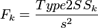
where
 is the
model variance. This statistic
reflects the change in the models' SSE that is the result of
removing the variable from the full model.
is the
model variance. This statistic
reflects the change in the models' SSE that is the result of
removing the variable from the full model.
- Type2SS statistic

This statistic estimates the importance of the variable by measuring the residual error change resulting from removing the variable from the model.
- Student t-statistic
The t-statistic for the k-th coefficient estimation
 is calculated as

where
 is the k-th diagonal element
of the matrix
is the k-th diagonal element
of the matrix
 .
.
- Variance Inflation Factor
The Variance Inflation Factor (VIF) statistic is defined as:
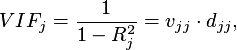
where
 is the
 statistics of the model which regresses variable
 on other explanatory variables,
 is the j-th diagonal element of
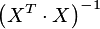 matrix, and
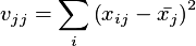
Table 37.4. Linear Regression Model Statistics: Model Fit Statistics
| Name | Description |
|---|---|
| AdjRsq |
the value of the adjusted coefficient of
determination
 |
| dfE |
the number of degrees of freedom for the SSE and MSE
statistics =
 , where
 is the number of observations
and
is the number of observations
and
 is the number of variables in
the model and
is the number of variables in
the model and
 accounts for the
optional
intercept.
accounts for the
optional
intercept.
|
| dfR | the number of degrees of freedom for the SSR and MSR statistics is equal to the number of variables in the model (taking into account the optional intercept term) |
| dfT | the number of degrees of freedom for the SST statistic is equal to the number of observations in the data |
| F-test | the value of the Fisher statistic |
| MSE | the mean residual error |
| MSR | the mean regression error |
| Pr>F |
the p-value for the
Fisher
statistic
for the model. The statistic has the Fisher
distribution with
 degrees of freedom, where
 is the number of observations,
 is the number of variables in
the model and
is the number of variables in
the model and
 accounts for the
optional
intercept.
accounts for the
optional
intercept.
|
| Rsq |
The value of the
 statistics
|
| SSE | the sum of squared errors |
| SSR | the sum of squared regression terms |
| SST | the total sum of squares |
| s | estimated model error standard deviance |
- AdjRsq statistic
The adjusted
 statistic is defined
as:
statistic is defined
as:

where
 is the number of observations in the
sample,
is the number of observations in the
sample,
 is the number of variables in the
model,
is the number of variables in the
model,
 for a model without intercept and
 for a model with an intercept (see
the
intercept
option).
for a model with an intercept (see
the
intercept
option).
- Fisher statistic
The Fisher statistic for the model is defined as:
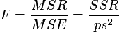
where p is the number of variables in the model and
 is the
model variance.
is the
model variance.
- MSE
The mean residual error is calculated as:
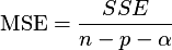 where n is the number of observations in the data and p is
the number of variables in the model and
where n is the number of observations in the data and p is
the number of variables in the model and
 accounts for the
optional
intercept.
accounts for the
optional
intercept.
- MSR
The mean regression error is calculated as:
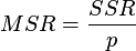 where p is the number of variables in the model.
-
Rsq (
 )
)
Associated with multiple regression the residual
 statistic is defined as:
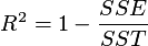 .
.
 is the coefficient of multiple
correlation, which reflects the percent of variance in the
dependent variable explained collectively by all of the
independent variables.
is the coefficient of multiple
correlation, which reflects the percent of variance in the
dependent variable explained collectively by all of the
independent variables.
-
Variance (
 )
)
The model variance is calculated as:
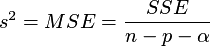
- SSE
The Sum of Squared Errors statistic is defined as the sum of square differences between the observed value of the dependent variable
 and predicted (regressed) value of
the dependent variable
and predicted (regressed) value of
the dependent variable
 :
:
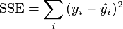
where
 is
the model fitted to the i-th value.
is
the model fitted to the i-th value.
- SSR
The regression error (Sum of Squared Regression) is defined as
 .
.
- SST
The variance of the dependent variable (The Total Sum of Squares) is defined as
 .
.
Table 37.5. Linear Regression Model Statistics: Group Statistics
| Name | Description | |
|---|---|---|
| Variable | the attribute name | |
| DF | number of degrees of freedom of variable or group of variables; in the second case numer of degrees is equal to the nuber of estimated parameters that means number of variables in group | |
| Wald Stat | the value of the residual (extra sum of squares) statistic, which compares the full model with a model from which a given variable is removed. | |
| Wald Pr>F | the p-value of the residual statistic | |
| Univariate Pr>F | the p-value of the Likelihood Ratio statistic for the model containing only the variable (or group of variables) (and optionally the intercept ). This statistic is calculated only if preselection = TRUE |
- Residual statistic
The residual statistic for a given variable is calculated according to the formula

where
 is the number of data samples,
 is the number of variables,
 if
intercept
is set to
TRUE and
if
intercept
is set to
TRUE and
 otherwise,
 is the
SSR statistic for the
full model,
is the
SSR statistic for the
full model,
 is the SSR statistic for the reduced model (without the
variable in question), and
is the SSR statistic for the reduced model (without the
variable in question), and
 is the
SSE statistic for the full model.
is the
SSE statistic for the full model.
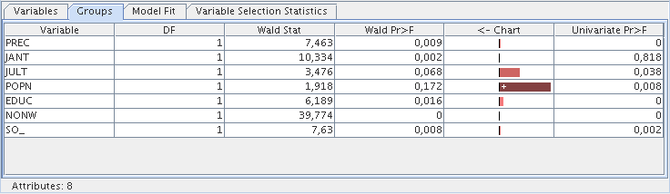
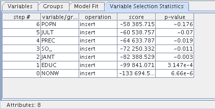
Table 37.6. Linear Regression Model Statistics: Variable Selection Statistics
| Name | Description |
|---|---|
| #step | iteration of variable selection algorithm |
| variable/group | the attribute (group of attributes) name |
| operation | action taken (remove / insert) due to variable during automatic variable selection process |
| score | value for the model-dependent Residual Statistic |
| p-value | the p-value for the model-dependent residual statistic |
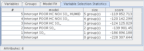
In the case of best subset variable selection algorithm the Variable Selection Statistics are differet.
Table 37.7. Linear Regression Model Statistics: Variable Selection Statistics: best subset
| Name | Description |
|---|---|
| # | iteration of variable selection algorithm |
| model | best model from models of the size |
| size | size of the model |
| score | the value of the model-dependent Scoring Statistic |
Additionally, the covariance and correlation matrices of the coefficient estimators as well as the correlation matrix of the attributes are calculated and displayed:
Table 37.8. Linear Regression Model Statistics: Coefficient / Attributes Correlation and Covariance
| Name | Description |
|---|---|
| Coefficient/ Attributes Correlation | the estimated data correlation matrix |
| Covariance Matrix | the estimated data covariance matrix |
- Correlation
The correlation matrix for the parameter estimators is calculated as

where
 are
the
are
the
 -th elements of the
covariance matrix
of the parameter estimators.
-th elements of the
covariance matrix
of the parameter estimators.
Correlation between attributes is calculated in standard way.
- Covariance Matrix
The covariance matrix for the parameter estimators is calculated as

where
 is the standard deviation of the
model,
is the standard deviation of the
model,
 is the vector of parameters and
 is the matrix of
independent variables.
is the matrix of
independent variables.
Note that both covariance and correlation matrices are symmetric and positively defined.
The estimated and tested model can be used for forecasting the dependent variable, model diagnostics and identifying outliers. The table below presents the possible output types and their descriptions.
To explain statistics below we need to introduce some notation. Let us define the HAT matrix as:

where X is matrix of independent variables,
 is the k-th diagonal element
of the HAT matrix. Let
is the k-th diagonal element
of the HAT matrix. Let  is the model
error variance without an k-th observation,
computed as:
is the model
error variance without an k-th observation,
computed as:

where  is an
error for k-th observation, and
is an
error for k-th observation, and
 accounts for the
optional intercept.
accounts for the
optional intercept.
Table 37.9. Approximation - Output items and output types combinations
| output type | output item type | description |
|---|---|---|
| predictedValue | aprox | returns the predicted value computed by the approximator |
| confidence | aprox | returns the probability that the approximated value is true. It depends on the particular algorithm how this value will be computed. Refer to the chapter describing the algorithm/module for more details. |
| cookDistance | linear regression |  ,
where
,
where
 accounts for the
optional
intercept.
accounts for the
optional
intercept.
|
| dfbetas | linear regression | DFBETAS statistics are calculated for each observation in apply data
and each attribute in the model signature. For each attribute v,
 column is created in the output table.
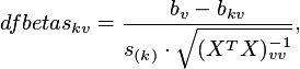  is
the v-th parameter estimate,
is
the v-th parameter estimate,
 is
is the v-th parameter estimate after deleting the k-th observation
is
is the v-th parameter estimate after deleting the k-th observation
|
| dffits | linear regression |  |
| leverage | linear regression |  |
| press | linear regression | 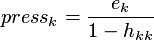 |
| rstudentResidual | linear regression |  |
| studentResidual | linear regression |  |