This section explains various attribute statistics available in the Freq component.
Basic attribute statistics are calculated for numerical attributes only. They are available via the Statistics display mode of an attribute in the Freq component.
Freq calculates the following statistics to provide a rough overview of the distribution of attribute values:
Minimum value. This is the smallest value attained by the attribute
Maximum value. This is the largest value attained by the attribute
1st quartile. This is a number which splits the samples into two parts: samples with values below the 1st quartile constitute 1/4 of of the dataset, samples with values above the 1st quartile constitute 3/4 of the dataset.
Median value. This is a number which splits the samples into two equal parts: samples with values below and above the median constitute respectively 1/2 of the value set. Median value is also called 2nd quartile.
3rd quartile. This is a number which splits the samples into two parts: samples with values below the 3rd quartile constitute 3/4 of of the dataset, samples with values above the 3rd quartile constitute 1/4 of the dataset.
Note
The minimum and maximum value statistics are different from Min and Max values in Intervals mode settings for an attribute.
For a numerical attribute  let
let  denote the number of samples and
  the
value of the
the
value of the  -th sample.
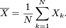
The variance (2nd moment) of an attribute is calculated as
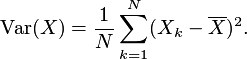
Variance measures how far the values of an attribute are spread out from the mean.

The skewness (3rd standardized moment) of an attribute is calculated as

Positive skewness indicates that the bulk of the samples lie mostly to the right of the mean, negative skewness means that there are more samples to the left of the mean.
The excess curtosis of an attribute is the ratio of the fourth moment about the mean by the square of the variance minus 3. It is calculated as

Positive values of excess kurtosis indicate that the density of the attribute has a thin and high peak near the mean and its tails are fatter. Negative values of excess curtosis indicate that the density peak around the mean is lower and broader, and the tails are thinner. Normal distributions have excess kurtosis equal to 0.
Attribute correlation statistics are available in the Correlation matrix component.
Pearson's correlation coefficient  calculated for two numerical attributes is
a popular measure of attribute interdepence. It assumes values between -1
and 1, the value of 1 corresponds to perfect positive linear dependence
between attributes, while the value of -1 corresponds to negative linear
dependece.
calculated for two numerical attributes is
a popular measure of attribute interdepence. It assumes values between -1
and 1, the value of 1 corresponds to perfect positive linear dependence
between attributes, while the value of -1 corresponds to negative linear
dependece.
Let  denote the sample size,
  ,
,  the values of the
  -th sample.
Pearson's correlation coefficient is calculated as
-th sample.
Pearson's correlation coefficient is calculated as

Correlation ratio is a measure of dependece between a
categorical variable
 and a numerical variable
  , defined as the ratio of two standard deviations
representing respectively the statistical dispersion of
, defined as the ratio of two standard deviations
representing respectively the statistical dispersion of  within
individual categories of
within
individual categories of  and the dispersion of
  across the whole sample.
Assume that the variable  is divided into categories
  and for each category
  the variable
  attains the values
  (here
(here
 is the number of samples in the category
  ). Let
  be the total sample count.
For a given category  define
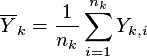
as the average of  restricted to the category
  .
.
The weighted standard deviation of category means is defined as
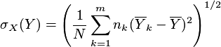
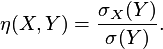
The correlation ratio  between
  and
and  is calculated as
In the calculation of correlation ratio matrix, if  is a numerical attribute attaining at most 100 distinct values, it will
be treated as categorical, with each value corresponding to one category. If the number of
different values exceeds 100, the correlation ratios with
is a numerical attribute attaining at most 100 distinct values, it will
be treated as categorical, with each value corresponding to one category. If the number of
different values exceeds 100, the correlation ratios with  as the categorical
variable will not be calculated.
as the categorical
variable will not be calculated.
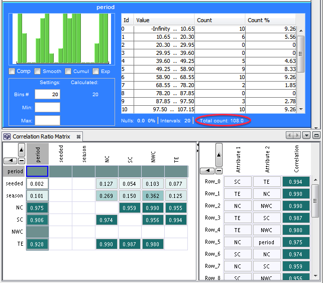
The correlation ratio matrix in the figure above has been calculated with rows treated as categorical variables. The numerical attribute period attains more than 100 values, hence the corresponding row does not contain any values.
Select or from the context menu to choose whether the variables corresoponding respectively to rows or columns are treated as categorical in the calculation of the correlation ratio statistics.
There are three statistics associated with Cramer's V-correlation: the Chi-Square coefficident, Crammer's coefficient and P-value.
The Chi-Square statistic can be treated as a measure of independence of
two categorical variables  and
and  .
.
Assume that  is divided
into
is divided
into  categories
  with counts
  and
and  is divided
into
is divided
into  categories
  with counts
  ,
,
 denotes the number of observations
for which the value of
denotes the number of observations
for which the value of  belongs to
  and the value of
  belongs to
  . Let
. Let
 be the total sample size.
The theoretical frequency for a given pair of categories  is calculated as

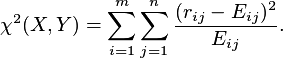
The value of the Chi-Square statistic is then calculated as
 the Cramer's coefficient
  assumes values between 0 and 1. The
value of
assumes values between 0 and 1. The
value of  corresponds to no association between variables and
  to complete
association.
to complete
association.

 assuming that
  and
and
 are independent.
For an attribute
 let
let  be the number of levels and
  be the index of the level.
The BeingGood value for the level  of the attribute
  is calculated according to the formula

where
 is the
number of records in the dataset for which the
value of the attribute
is the
number of records in the dataset for which the
value of the attribute  belongs to the
 -th
level and is not the positive target value.
-th
level and is not the positive target value.
 is the
number of records in the dataset for which the
value of the attribute
is the
number of records in the dataset for which the
value of the attribute  belongs to the
 -th
level and is the positive target value.
-th
level and is the positive target value.
 is the total
number of records in the training dataset for which the
value of the attribute
is the total
number of records in the training dataset for which the
value of the attribute  is not
the positive target value.
is not
the positive target value.
 is the total
number of records in the training dataset for which the
value of the attribute
is the total
number of records in the training dataset for which the
value of the attribute  is
the positive target value.
is
the positive target value.
The Weight of Evidence statistic for the  -th level of the attribute
  is calculated as

 is calculated as
