Table of Contents
The Distributions Library provides tools for using common distributions: calculating their characteristics (like mean, median, variance, density function etc.) and generating their samples.
The AdvancedMiner offers the following methods for calculating the characteristics of the implemented distributions and generating their samples.
Table 20.1. Available methods
| Method | Description |
| cdf(x double) | returns the value of the cumulative distribution function at the point x |
| estimateDistribution(_sample) | estimates the parameters of the distribution based on the data sample _sample |
| kurtosis() | returns the value of the kurtosis |
| mean() | returns the value of the mean |
| median() | returns the value of the median |
| mode() | returns the modal value |
| pdf(x double) | returns the value of the probability density function at point x |
| quantile(p double) | returns the value of the p-th quantile |
| rand() | returns a pseudo-random number with the given distribution |
| skewness() | returns the value of the skewness |
| standardDeviation() | returns the value of the standard deviation |
| variance() | returns the value of the variance |
Not all the methods listed above are implemented for each distribution. However it is possible to check whether the given method is supported by the given distribution class using the supportsCapability method (see the example below).
Example 20.1. Using distributions library (poisson distribution)
from biz.sc.math.distributions import *
from biz.sc.math.distributions.discrete import *

_lambda = 3

_Poi  = PoissonDistribution(_lambda)
_Poi.setSeed(1245)

print 'Mean: ',_Poi.mean()
print 'Variance: ',_Poi.variance()
print 'Mode: ',_Poi.mode()
print 'Propability density function: ',_Poi.pdf(3)
print 'Standard deviation:',_Poi.standardDeviation()
print 'Supports estimation:',_Poi.supportsCapability(biz.sc.math.distributions.DistributionCapability.estimation)
Output:
Mean:  3.0
Variance:  3.0
Mode:  3.0
Propability density function:  0.22404180765538775
Standard deviation: 1.7320508075688772
Supports estimation: 1
Beta distribution is a continuous probability distribution with a density function on real line given by the formula

A Beta Distribution object may be created in one of the following ways:
BetaDistribution(p, q) - creates a new beta distribution object with a lower bound min = 0, an upper bound max = 1 and shape parameters p and q.
BetaDistribution(max, p, q) - creates a new beta distribution object with a lower bound min = 0, an upper bound max and shape parameters p and q.
BetaDistribution(min, max, p, q) - creates a new beta distribution object with a lower bound min, an upper bound max and shape parameters p and q.
Table 20.2. BetaDistribution parameters
Parameter Type of the parameter min double max double p positive double q positive double Table 20.3. Specific methods for the beta distribution
Method Description getMax() returns the value of the parameter max getMin() returns the value of the parameter min getP() returns the value of the parameter p getQ() returns the value of the parameter q setMax() sets the value of the parameter max setMin() sets the value of the parameter min setP() sets the value of the parameter p setQ() sets the value of the parameter q Chi-Square distribution is a special case of the gamma distribution which has the density function on the real line given by the formula

ChiSquareDistribution(df) creates a new chi-square distribution object with df degrees of freedom.
Erlang distribution is a case of the gamma distribution with a density function on the real line given by the formula

ErlangDistribution(alpha) creates a new Erlang distribution object with the location parameter gamma = 0, the scale parameter beta = 1 and the shape parameter alpha.
ErlangDistribution(beta, alpha) creates a new Erlang distribution object with the location parameter gamma = 0, the scale parameter beta and the shape parameter alpha.
ErlangDistribution(gamma, beta, alpha) creates a new Erlang distribution object with the location parameter gamma, the scale parameter beta and the shape parameter alpha.
Table 20.6. Parameters of ErlangDistribution
Parameter Type of the parameter gamma double beta positive double alpha positive integer Table 20.7. Specific methods for the Erlang distribution
Method Description getAlphai() returns the value of the parameter alpha getBeta() returns the value of the parameter beta getGamma() returns the value of the parameter gamma setAlphai() sets the value of the parameter alpha setBeta() sets the value of the parameter beta setGamma() sets the value of the parameter gamma Exponential distribution is a case of the Erlang distribution (corresponding to h = 1) with a density function on the real line given by the formula
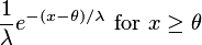
ExponentialDistribution() creates a new exponential distribution object with the scale parameter lambda = 1 and the location parameter theta = 0.
ExponentialDistribution(lambda) creates a new exponential distribution object with the scale parameter lambda and the location parameter theta = 0.
ExponentialDistribution(lambda , theta) creates a new exponential distribution object with the scale parameter lambda and the location parameter theta.
Fisher distribution is a continuous probability distribution with a density function on the real line given by the formula

FDistribution(nu_1 , nu_2) creates a new Fisher distribution object with shape parameters nu_1 and nu_2.
Gamma distribution is a continuous probability distribution with a density function on the real line given by the formula

GammaDistribution(alpha) creates a new gamma distribution object with the location parameter gamma = 0, the scale parameter beta = 1 and the shape parameter alpha.
GammaDistribution(beta, alpha) creates a new gamma distribution object with the location parameter gamma = 0, the scale parameter beta and the shape parameter alpha.
GammaDistribution(gamma, beta, alpha) creates a new gamma distribution object with the location parameter gamma, the scale parameter beta and the shape parameter alpha.
Table 20.12. Parameters of GammaDistribution
Parameter Type of the parameter theta double lambda positive double alpha positive double Table 20.13. Specific methods for the gamma distribution
Method Description getAlpha() returns the value of the parameter alpha getBeta() returns the value of the parameter beta getGamma() returns the value of the parameter gamma setAlpha() sets the value of the parameter alpha setBeta() sets the value of the parameter beta setGamma() sets the value of the parameter gamma Inverse chi-square distribution is a continuous probability distribution with a density function on the real line given by the formula

InverseChiSquaredDistribution(double df) creates an Inverse chi-square distribution object with df degrees of freedom.
Inverse gamma distribution is a continuous probability distribution with a density function on real line given by the formula

InverseGammaDistribution(alpha) creates a new inverse gamma distribution object with the location parameter gamma = 0, the scale parameter beta = 1 and the shape parameter alpha.
InverseGammaDistribution(beta, alpha) creates a new inverse gamma distribution object with the location parameter gamma = 0, the scale parameter beta and the shape parameter alpha.
InverseGammaDistribution(gamma, beta, alpha) creates a new Inverse gamma distribution object with the location parameter gamma, the scale parameter beta and the shape parameter alpha.
Table 20.16. Parameters of Inverse GammaDistribution
Parameter Type of the parameter gamma double beta positive double alpha positive double Table 20.17. Specific methods for the inverse gamma distribution
Method Description getAlpha() returns value of the parameter alpha getBeta() returns value of the parameter beta getGamma() returns value of the parameter gamma setAlpha() sets value of the parameter alpha setBeta() sets value of the parameter beta setGamma() sets value of the parameter gamma Multivariate normal distribution is a continuous probability distribution with a density function on n-dimensional real vector space given by the formula

MultivariateNormalDistribution(n) creates a new n - dimensional multivariate normal distribution object with the location vector mean mu = 0 and the covariance matrix = identity matrix.
MultivariateNormalDistribution(Sigma) creates a new multivariate normal distribution object with the location vector mean mu = 0 and the covariance matrix Sigma.
MultivariateNormalDistribution(Mean, Sigma) creates a new multivariate normal distribution object with the location vector mean mu and the covariance matrix Sigma.
Table 20.18. Parameters of MultivariateNormalDistribution
Parameter Type of the parameter mu n - dimensional vector of reals Sigma positive definite, symmetric n x n-dimensional matrix of real numbers n positive integer Table 20.19. Specific methods for the multivariate normal distribution
Method Description covariance() returns the covariance matrix Sigma dim() returns the dimension n mean() returns the mean vector mu setCovariance() sets the covariance matrix Sigma setDim() sets the dimension n setMean() sets the mean vector mu Normal distribution is a continuous probability distribution with a density function on the real real line given by the formula
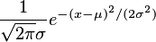
NormalDistribution() creates a new normal distribution object with mean mu = 0 and variance sigma = 1.
NormalDistribution(sigma) creates a new normal distribution object with mean mu = 0 and variance sigma.
NormalDistribution(mu, sigma) creates a new normal distribution object with mean mu and variance sigma.
Pareto distribution is a continuous probability distribution with a density function on the real line given by the formula

ParetoDistribution(alpha) creates a new Pareto distribution object with the location-scale parameter xmin =1 and the scale parameter alpha.
ParetoDistribution(xmin, alpha) creates a new Pareto distribution object with the location-scale parameter xmin and the scale parameter alpha.
Student's t-distribution is a continuous probability distribution with a density function on the real line given by the formula

StudentsTDistribution(nu) creates a new Student's t distribution object with the location parameter theta = 0, the scale parameter lambda = 1 and the shape parameter nu.
StudentsTDistribution(lambda, nu) creates a new Student's t distribution object with the location parameter theta = 0, the scale parameter lambda and the shape parameter nu.
StudentsTDistribution(theta, lambda, nu) creates a new Student's t distribution object with the location parameter theta, the scale parameter lambda and the shape parameter nu.
Table 20.23. Parameters of StudentsTDistribution
Parameter Type of the parameter theta double lambda positive double nu positive integer Table 20.24. Specific methods for the Student's t-distribution
Method Description getLambda() returns the value of the parameter lambda getNu() returns the value of the parameter nu getTheta() returns the value of the parameter theta setLambda() sets the value of the parameter lambda setNu() sets the value of the parameter nu setTheta() sets the value of the parameter theta Uniform distribution is a continuous probability distribution with a density function on the real line given by the formula

UniformDistribution() creates a new uniform distribution object with the lower bound = 0 and the upper bound = 1.
UniformDistribution(min, max) creates a new uniform distribution object with the lower bound = min and the upper bound = max.
Binomial distribution is a discrete probability distribution with a density function given by the formula

BinomialDistribution(n, p) creates a new binomial distribution object with the number of trials parameter n and the success probability parameter p.
Geometric distribution is a discrete probability distribution with a density function given by the formula

GeometricDistribution(p) creates a new geometric distribution object with the probability parameter p.
Poisson distribution is a discrete probability distribution with a density function given by the formula

PoissonDistribution(lambda) creates a new Poisson distribution object with the frequency parameter lambda.
Example 20.3. Using distributions library (normal distribution)
#Example for using Distributions Library

from biz.sc.math.distributions import *

from biz.sc.math.distributions.continuous import *

_mu = 0.3
_sigma = 0.1

_norm = NormalDistribution(_mu, _sigma)
_norm.setSeed(1222)

print 'Mean: ',_norm.mean()
print 'Skewness: ',_norm.skewness()
print 'Kurtosis: ',_norm.kurtosis()

print 'Cumulative distribution function: ',_norm.cdf(0.2)
print 'Propabilty density function:',_norm.pdf(0.2)

print 'Cumulative distribution function (quantile):',_norm.cdf(_norm.quantile(0.2))
Output:
Mean:  0.3
Skewness:  0.0
Kurtosis:  0.0
Cumulative distribution function:  0.15865526139567465
Propabilty density function: 2.419707245191434
Cumulative distribution function (quantile): 0.19999999817822584
AdvancedMiner offers tables of distributions which frequently appear in statistical tests such as Anderson Darling or Kolmogorov-Smironov tests. Tables are objects of DistributionsTablesFactory class and specific distribution tables are instances of the tables (see the example below).
Example 20.4. Using distributions library (normal distribution)
from biz.sc.math.distributions.tables import *

_table = DistributionTablesFactory.getInstance()

_Ftable = _table.getFCriticalValuesInstance()

print 'Quantile:',_Ftable.quantile(.09, 2,3)
Output:
Quantile: 5.46238
The table below there list the available tables and their constructors.
Table 20.33. Available tables and their constructors
| Table | Construction Method | |
| getADA2CriticalValuesInstance() | Percentage points for the modified Anderson-Darling A^2 statistics | |
| getADA2LogisticCriticalValuesInstance() | Anderson-Darling A^2 tests for the logistic distribution critical values | |
| getChiSquareCriticalValuesInstance() | Upper critical values of the chi-square distribution for a one-sided chi-square test | |
| getFCriticalValuesInstance() | Upper critical values of the F-distribution for one-sided F test | |
| getKS2SampleTableInstance() | Kolmogorov-Smirnov distribution critical values table for two samples | |
| getKSPValuesInstance() | The cumulative distribution function for the Kolmogorov-Smirnov statistics | |
| getKSTableInstance() |
| |
| getStudentsTCriticalValuesInstance() | Upper critical values of Student's t distribution with df degrees of freedom |
Percentage points for the modified Anderson-Darling A^2 statistics
The Anderson-Darling statistics is described in the chapter Statistical Procedures and Tests.
Table 20.34. Methods offered by the table
Method Description quantile(double upperTailPP) returns the quantile for F(x) completely known, upperTailPP - the upper tail percentage point (0.85, 0.90, 0.95, 0.975, 0.99) quantile(double upperTailPP, int modCode) returns the quantile for modified F(x) depending on modCode - the modification code (0, 3, 4), 0 for sample size >= 5 and F(x) completely known, 3 for testing normality with mean and variance unknown, 4 for testing exponentiality with mean unknown, and upperTailPP - upper tail percentage point (0.85, 0.90, 0.95, 0.975, 0.99) quantileApprox(double upperTailPP) approximates the quantile for F(x) completely known using the equation p = ln(1-upperTailPP), criticalValue = 0.164111752625 + p * (-0.719787337528 + p * 0.020207904162) Anderson-Darling A^2 test for the logistic distribution critical values
The Anderson-Darling statistics is described in the chapter Statistical Procedures and Tests.
Table 20.35. Methods offered by the table
Method Description quantile(double upperTailPP) returns the quantile for F(x) completely known, upperTailPP - the upper tail percentage point (0.85, 0.90, 0.95, 0.975, 0.99) quantile(double upperTailPP, int modCode) returns the quantile for modified F(x), depending on modCode - the modification code (0, 1, 2, 3), 0 for no modification, 1 for A^2_mod = A^2+0.15/n, 2 for A^2_mod = (0.6nA^2-1.8)/(0.6/n-1.0), 3 for A^2_mod = A^2(1.0 + 0.25/n), upperTailPP - the upper tail percentage point (0.85, 0.90, 0.95, 0.975, 0.99) Upper critical values of the chi-square distribution for one-sided chi-square test
The chi-square statistics is described in the chapter Statistical Procedures and Tests.
Upper critical values of the F-distribution for one-sided F test
The F statistics is described in the chapter Statistical Procedures and Tests.
Kolmogorov-Smirnov distribution critical values table for two samples
The Kolmogorov-Smirnov test for two samples is described in the chapter Statistical Procedures and Tests.
The cumulative distribution function for Kolmogorov-Smirnov statistics
The Kolmogorov-Smirnov test is described in the chapter Statistical Procedures and Tests.
Kolmogorov-Smirnov statistics' critical values
The Kolmogorov-Smirnov test is described in the chapter Statistical Procedures and Tests.
Upper critical values of Student's t distribution with df degrees of freedom
Student's t statistics is described in chapter Statistical Procedures and Tests.