There are two types of tests in hypothesis testing: parametric and non-parametric. Traditional tests are called parametric because they need a specification of an underlying probability distribution (except for the free parameters). It means that the distribution type and the distribution parameters should be precisely specified. Parametric tests depend on these assumptions about the probability distribution. Non-parametric tests do not require any assumptions about the distributions.
The following conditions should be met for proper hypothesis testing:
The data set is drawn from a random sample.
The observations are independent of each other.
Statistical test procedures use numerical data sets which can have two types of representation:
For the standard type representation separate data sets are stored in the data table in separate columns. For the key-type representation the two data sets are stored in one 'united' column while an additional key column indicates the sample for the particular element. The key column must contain a variable with only two possible outcomes (either categorical or numerical).
Null (missing) values in the data set are supported and the missed observations are omitted.
All statistical tests are accessible from the script level. In order to apply a particular statistical test to sample data a script should be created.
The following commands are used for implementing the tests:
runStatTest(test, table)  or
runStatTest(test, table, col1)  or
runStatTest(test, table, col1, col2)
The general form of the command is
runStatTest(test, alias.table, col1, col2)
where
test is the name of the object representing the corresponding statistical test,
alias is the name of an alias pointing to a database. This parameter is optional, if omitted the default alias will be used
table is the name of the table in the database indicated by the alias where the data samples for testing are stored,
col1 is the name of the first column to be used in the test,
col2 is the name of the second column to be used in the test.
If no column names are given, the test procedure will take the first column from the specified table and try to implement the test.
The test object is created in two steps:
1) creating the corresponding test settings
2) creating the selected test object using the commands:
settings = TestNameSettings()
test = TestName(settings)
where settings and test are the names of the corresponding objects.
A list of all elements of settings for each statistical test can be found in the Settings section for the corresponding test. TestName /TestNameSettings can be any of the following:
The results of the test are stored as an object with the chosen name:
res = runStatTest(test, alias.table, col1, col2)
Here res is the name of the resulting object of the test implementation for the set (test, alias.table, col1, col2) . The result of the test contains four elements: the value of the test statistic, the critical value(s) for the given significance level, the p-value for the calculated test statistic value and the resulting hypothesis (null hypothesis is rejected or accepted), which can be printed to the output window using the following commands:
res.printResults()
to print all results or
                    res.getHypothesis()
                    res.getStatistic()
                    res.getCriticalValue()
                    res.getPValue()
to extract the particular elements separately.
The getHypothesis() command prints the resulting hypothesis as 0/1, which corresponds to null hypothsis/alternative hypothesis.
Below is a list of all commands for the definition of the separate elements of a selected settings object (the default parameter values can be found in the settings table for each test):
Table 19.1. Statistical Tests Settings: Set Commands
| Name | Command |
|---|---|
| alpha | settings.setAlpha(value) |
| choice | settings.setChoice(StatcisticalTestsSettings.value) |
| distribution | settings.setDistributionType(StatisticalTestsSettings.value) |
| location | settings.setLocation(value) |
| low | settings.setLowerBound(value) |
| mZero | settings.setMZero(value) |
| meanZero | settings.setMeanZero(value) |
| pair | settings.setPair(StatisticalTestsSettings.value) |
| representation | settings.setRepresentation(StatisticalTestsSettings.value) |
| scale | settings.setScale(value) |
| shape | settings.setShape(value) |
| shape2 | settings.setShape2(value) |
| side | settings.setSide(StatisticalTestsSettings.value) |
| sigmaZero | settings.setSigmaZero(value) |
| up | settings.setUpperBound(value) |
| varEqual | settings.setVarEqual(StatisticalTestsSettings.value) |
The admissible values for each element of the settings can be found in the description of each test in the Settings section. For viewing the setting values the following commands can be used:
Table 19.2. Statistical Tests Settings: View Commands
| Name | Command |
|---|---|
| alpha | settings.getAlpha() |
| choice | settings.getChoice() |
| distribution | settings.getDistributionType() |
| location | settings.getLocation() |
| low | settings.getLowerBound() |
| meanZero | settings.getMeanZero() |
| mZero | settings.getAlpha() |
| pair | settings.getPair() |
| representation | settings.getRepresentation() |
| scale | settings.getScale() |
| shape | settings.getShape() |
| shape2 | settings.getShape2() |
| side | settings.getSide() |
| sigmaZero | settings.getSigmaZero() |
| up | settings.getUpperBound() |
| varEqual | settings.getVarEqual() |
Example 19.4. Mann Whitney Test
table 'statTest':
    a b

    1 2
    5 6
    1 7
    2 4
    5 8


settingsMW = MannWhitneyTestSettings()
settingsMW.setAlpha(0.1)
testMW = MannWhitneyTest(settingsMW)
resMW = runStatTest(testMW, 'statTest', 'a', 'b')
resMW.printResults()
Output:
        StatTestResult:

        1) Critical value:         1.6448536269514715
        2) Statistic:        -1.6711454971746993
        3) p-value:        0.09469293918766253
        4) Hypothesis:        null hypotesis is rejected
Some tests described below are based on the empirical distribution
function (EDF)
 , which is defined as follows:

where
 are the ordered distinct observations.
The Anderson-Darling test (Anderson and Darling 1954, Stephens 1974) is a modification of the Kolmogorov-Smirnov (KS) test and is used to test whether a data sample comes from a population with a specified distribution. The KS test is distribution free in the sense that the critical values do not depend on the specific distribution being tested. By contrast, the critical values for the Anderson-Darling test are dependent on the specific distribution that is being tested. This has the advantage of allowing a more sensitive test and the disadvantage that critical values must be calculated for each distribution.
The Anderson-Darling test is defined as:
Hypothesis:
The data sample is drawn from a population with the specified distribution.
The data sample is drawn from a population with another distribution.
Test Statistic: The Anderson-Darling test statistic is defined as

and is calculated as
 ,
where
,
where

Here  are the ordered data and
 is the sample size,
 is the cumulative distribution function of the
specified distribution,
is the cumulative distribution function of the
specified distribution,
 is the empirical distribution function,
which estimates the distribution function
is the empirical distribution function,
which estimates the distribution function
 .
.
For every  the value
  is the proportion of observations
less than or equal to
is the proportion of observations
less than or equal to  , while
  is the probability of an observation
less than or equal to
is the probability of an observation
less than or equal to  .
.

The test is a one-sided test and the hypothesis that the distribution is of a specific form is rejected if the test statistic A is greater than the critical value.
The critical values for the Anderson-Darling test are dependent on the specific distribution that is being tested. Tabulated values and formulas have been published (Stephens 1974, 1976, 1977, 1979) for a few specific distributions (normal, lognormal, exponential, Weibull, logistic, extreme value type 1 (Gumbel)).
Note
The Anderson-Darling statistic may be multiplied by a constant (which usually depends on the sample size). These constants are given in various papers by Stephens.
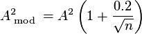
The normal and lognormal distributions require the following modification for small samples:

Then the test statistic has to be compared to the appropriate critical value.
For the Weibull and Gumbel distributions the test statistic for small samples is calculated as follows:
As for the exponential distribution, it is a special case of the Weibull distribution with the scale parameter equal to the mean parameter of the exponential distribution and the shape parameter equal to 1.
The probability of a larger test statistic is obtained by linear interpolation within the range of the simulated critical values (see D'Agostino and Stephens 1986).
The P-value is equal to the probability of a random variable with Andeson-Darling distribution to be greater than or equal to the observed value of the AD statistic under the null hypothesis.
Data Requirements:
The Anderson-Darling test is performed for one sample of numerical data, which can be stored either in one column (standard representation) or in two columns (key-type representation).
Table 19.3. Anderson-Darling Test Settings
| Name | Description | Possible values | Default value |
|---|---|---|---|
| alpha | confidence level | real numbers from the interval (0,0.25) | 0.05 |
| distribution | distribution type | DISTRIBUTION_NORMAL, DISTRIBUTION_EXPONENTIAL, DISTRIBUTION_BETA, DISTRIBUTION_GAMMA, DISTRIBUTION_LOGISTIC | DISTRIBUTION_NORMAL |
| location | location parameter for the selected distribution | real numbers | 0 |
| low | lower bound parameter for the Beta distribution | real numbers | 0 |
| representation | data sample representation type | STANDARD_REPRESENTATION, SAMPLE_KEY_REPRESENTATION | STANDARD_REPRESENTATION |
| scale | scale parameter for the selected distribution | positive real numbers | 1 |
| shape | shape parameter for the selected distribution | positive real numbers | 1 |
| shape2 | second shape parameter for the Beta distribution | positive real numbers | 1 |
| up | upper bound parameter for the Beta distribution | real numbers | 1 |
Table 19.4. Anderson-Darling Test Settings: Set Commands and View Commands
| Name | Set Command | View Command |
|---|---|---|
| alpha | settings.setAlpha(value) | settings.getAlpha() |
| distribution | settings.setDistributionType(StatisticalTestsSettings.value) | settings.getDistributionType() |
| location | settings.setLocation(value) | settings.getLocation() |
| low | settings.setLowerBound(value) | settings.getLowerBound() |
| representation | settings.setRepresentation(StatisticalTestsSettings.value) | settings.getRepresentation() |
| scale | settings.setScale(value) | settings.getScale() |
| shape | settings.setShape(value) | settings.getShape() |
| shape2 | settings.setShape2(value) | settings.getShape2() |
| up | settings.setUpperBound(value) | settings.getUpperBound() |
Example 19.5. Anderson Darling test
#  Anderson-Darling test example


table 'Anderson_Darling':
    a

    1.3
    1.5
    1.2
    1.2
    1.5
    1.3
    1.4
    1.3
    1.5

settings = AndersonDarlingTestSettings()
settings.setAlpha(0.1)
settings.setLocation(0.2)
test = AndersonDarlingTest(settings)

res = runStatTest(test, 'Anderson_Darling')

res.printResults()
Output:
        StatTestResult:

        1) Critical value:         1.933
        2) Statistic:        9.962506280437683
        3) p-value:        Could not calculate p-Value, exact message is: Not implemented for Anderson-Darling test.
        4) Hypothesis:        null hypotesis is rejected
The above example performs the Anderson-Darling test for the sample 'a'. The null hypothesis here is that the sample data set 'a' conforms to the normal distribution with mean 0.2 and unit standard deviation. At the 0.1 level the null hypothesis is rejected.
The Chi-square test can be used to test whether the variance of a population is equal to a predetermined value.
The data requirements for the version of the chi-square test implemented in AdvancedMiner are: the data set is drawn from a normally distributed random sample with known mean and unknown variance.
This test can be either two-sided test or one-sided. The two-sided version tests against the alternative that the true variance is not equal to the specified value. The one-sided version tests only in one direction: the true variance is less than the predetermined value (left-sided test) or the true variance is greater than the predetermined value (right-sided test). The choice of the two-sided versus one-sided test is determined by the problem.
Hypothesis:
The population variance is equal to
.

Two-sided test: The population variance is not equal to
.
Left-sided test: The population variance is less than
.
Right-sided test: The population variance is greater than
.
Test Statistic:
The test statistic has the form
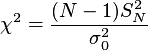
where  is the sample size and
  is the sample variance. It can be seen
from this formula that the test compares the ratio of the sample
variance to the target variance. The more this ratio deviates from 1,
the more likely we are to reject the null hypothesis.
is the sample variance. It can be seen
from this formula that the test compares the ratio of the sample
variance to the target variance. The more this ratio deviates from 1,
the more likely we are to reject the null hypothesis.
Under the null hypothesis the test statistic has a chi-square
distribution with  degrees of freedom.

The null hypothesis is rejected if:
Two-sided test :

Left-sided test :
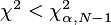
Right-sided test :

Here  and
and  are respectively the lower
and upper quantile of a chi-square distribution with
are respectively the lower
and upper quantile of a chi-square distribution with
 degrees of freedom.
The P-value is equal to the probability that a random variable
with a chi-square distribution with  degrees of freedom will be greater or
equal to the calculated value of the test statistic under the null
hypothesis.
degrees of freedom will be greater or
equal to the calculated value of the test statistic under the null
hypothesis.
Data Requirements:
The Chi-square test can be performed for numerical samples in the standard or key-type representations.
Table 19.5. Chi-square Test Settings
| Name | Description | Possible values | Default value |
|---|---|---|---|
| alpha | confidence level | real numbers from the interval (0,0.5) | 0.05 |
| representation | data sample representation type | STANDARD_REPRESENTATION, SAMPLE_KEY_REPRESENTATION | STANDARD_REPRESENTATION |
| side | the type of the test | TWO_SIDED, LEFT_SIDED, RIGHT_SIDED | TWO_SIDED |
| sigmaZero | the value of the variance for the null hypothesis | real numbers | 1 |
Table 19.6. Chi-square Test Settings: Set Commands and View Commands
| Name | Set Command | View Command |
|---|---|---|
| alpha | settings.setAlpha(value) | settings.getAlpha() |
| representation | settings.setRepresentation(StatisticalTestsSettings.value) | settings.getRepresentation() |
| side | settings.setSide(StatisticalTestsSettings.value) | settings.getSide() |
| sigmaZero | settings.setSigmaZero(value) | settings.getSigmaZero(value) |
Example 19.6. Chi square test
# Chi-square test example


table 'chi_square':
    s1 s2

    1  3
    5  3
    1  3
    2  3
    5  3
    3  3
    4  3
    5  3
    2  3
    1  3

settings = ChiSquareTestSettings()
settings.setAlpha(0.1)
settings.setSigmaZero(2)
test = ChiSquareTest(settings)

settings.setSide(StatisticalTestsSettings.LEFT_SIDED)

res = runStatTest(test, 'chi_square', 's1')
res.printResults()
Output:
        StatTestResult:

        1) Critical value:         4.168159042550835
        2) Statistic:        6.724999999999999
        3) p-value:        0.3342739213749686
        4) Hypothesis:        null hypotesis is accepted
The above example performs the chi-square test for the sample data "s1" and checks whether the data conforms with the assumption that the population variance is equal to 2. This hypothesis is rejected at the level of confidence of 0.1.
The F-test (Snedecor and Cochran 1989) is used to test whether the standard deviations of two populations are equal.
The following assumptions should be met:
1. The two data samples are drawn from the same normal distribution (i.e.for each sample the values are independent and identically normally distributed).
2. The two samples are independent of each other.
There are two versions of this test: two-tailed and one-tailed. The two-tailed test is used to test whether standard deviations are equal. The one-tailed version tests in one direction: the left-sided variant checks whether the standard deviation for the first population is less than the one for the second population and the right-sided variant checks whether the standard deviation for the first population is greater than the one for the second population. The choice is determined by the problem.
The F-test checks the ratio of the variances of the two samples. The more this ratio deviates from 1, the more likely the null hypothesis will be rejected.
Hypothesis:
The two populations have equal variances.

Two-sided test: The two populations do not have equal variances.
Left-sided test: The standard deviation of the first population is less than the standard deviation of the second population.
Right-sided test: The standard deviation of the first population is greater than the standard deviation of the second population.
Test Statistic:
The F-test statistic has the following form:

where  is the variance of the first sample
and
is the variance of the first sample
and  is the variance of the second
sample.
is the variance of the second
sample.
As seen from this formula the F-test checks the ratio of the variances of the two samples . The more this ratio deviates from 1, the more likely the null hypothesis will be rejected.

The null hypothesis is rejected if:
Two-sided test :

Left-sided test :

Right-sided test:

where  are the
quantiles of an F-distribution with
are the
quantiles of an F-distribution with  degrees of freedom,
 is the first sample size and
 is the second sample size.
Under the null hypothesis the P-value is equal to the
probability that a random variable with a Fisher-Snedecor
F-distribution with  degrees of freedom will
be greater or equal to the calculated value of the test
statistic
degrees of freedom will
be greater or equal to the calculated value of the test
statistic
Data Requirements:
The F-test is performed for two numerical data samples which can have a standard or key-type representation.
| Name | Description | Possible values | Default value |
|---|---|---|---|
| alpha | confidence level | real number from the interval (0,0.5) | 0.05 |
| representation | data sample representation type | STANDARD_REPRESENTATION, SAMPLE_KEY_REPRESENTATION | STANDARD_REPRESENTATION |
| side | the type of the test | TWO_SIDED, LEFT_SIDED, RIGHT_SIDED | TWO_SIDED |
Table 19.8. F-Test Settings: Set Commands and View Commands
| Name | Set Command | View Command |
|---|---|---|
| alpha | settings.setAlpha(value) | settings.getAlpha() |
| representation | settings.setRepresentation(StatisticalTestsSettings.value) | settings.getRepresentation() |
| side | settings.setSide(StatisticalTestsSettings.value) | settings.getSide() |
Example 19.7. F-test
# F-test example
table 'FTest':
    f1 f2

    1 2
    5 1
    1 5
    2 1
    5 5
    3 4
    2 3
    4 2

settings = FTestSettings()
test = FTest(settings)

res = runStatTest(test, 'FTest', 'f1', 'f2')
res.printResults()
Output:
        StatTestResult:

        1) Critical value:         0.2002038387771814                4.994909219063272
        2) Statistic:        1.0
        3) p-value:        0.9999999940600666
        4) Hypothesis:        null hypotesis is accepted
A frequently encountered problem is to verify that a predefined probability distribution represents the population of the data in question. In the 1930s Kolmogorov and Smirnov developed a goodness of fit test for continuous data to determine whether a sample comes from a given hypothesized distribution. Today it continues to be one of the best known and most widely used goodness of fit tests. This is due to its simplicity and because it is based on the empirical distribution function (EDF), which converges uniformly to the population's cumulative distribution function (CDF) with probability measure one (the Glivenko-Cantelli theorem). Even though a plethora of goodness of fit tests have been developed in recent decades (see for example, D'Agostino and Stephens 1986), many with higher statistical power than the Kolmogorov-Smirnov (KS) test, the KS test remains popular because it is simple and intuitive. The objective of the Kolmogorov-Smirnov test is to test whether a sample of a random variable belongs to a specific predefined distribution. The null hypothesis must therefore specify both the type of distribution function and its parameters. The alternative hypothesis is that the assumed probability distribution function does not match the underlying one. The idea behind the Kolmogorov-Smirnov test is quite simple: the maximum difference between the assumed CDF and EDF of the random sample to be investigated is used to decide whether the random sample belongs to the distribution or not. For a single sample of data, the Kolmogorov-Smirnov test is used to test whether or not the sample of data is consistent with a specified distribution function. When there are two samples of data, it is used to test whether or not these two samples may reasonably be assumed to come from the same probability distribution.
The Kolmogorov-Smirnov (KS) test is based on the empirical distribution function (EDF).
Hypothesis: One-sample test
The data follows a specified distribution.
The data does not follow the specified distribution.
Two-samples test:
The two empirical distributions coincide.
The two empirical distributions are different.
The following distributions are implemented: Normal, Exponential, Logistic distribution, Beta-distribution, Gamma-distribution.
Test Statistic:
The KS test statistic is defined as:
For the one-sample test:

where
 is the theoretical cumulative distribution
of the distribution being tested, which must be a continuous
distribution (i.e. no discrete distributions such as the binomial or
Poisson) and fully specified (i.e. all distribution
parameters should be specified, as in the test routine the
distribution parameters cannot be estimated from the data), and
is the theoretical cumulative distribution
of the distribution being tested, which must be a continuous
distribution (i.e. no discrete distributions such as the binomial or
Poisson) and fully specified (i.e. all distribution
parameters should be specified, as in the test routine the
distribution parameters cannot be estimated from the data), and
 is the EDF
for the sample.
is the EDF
for the sample.
Note
Due to the properties of EDF the one sample test statistic is computed according to the following formula:

where
 is the sample size,
 are the ordered distinct observations, and it is assumed that
 .
.
The asymptotic statisic value is obtained from the formula

For the two-samples test:

where  are the pulled ordered observations from
the two samples,
are the pulled ordered observations from
the two samples,  is the total sample size,
 is the first sample size,
 is the second sample size and
 and
and  are EDF-s for the first and second
sample accordingly.
are EDF-s for the first and second
sample accordingly.
The value of the asymptotic statisic is obtained from the equation
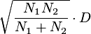

The null hypothesis is rejected if the calculated sample value of the KS test statistic greater than the corresponding critical value of the distribution of the Kolmogorov-Smirnov test statistic. This distribution depends on sample size and confidence level
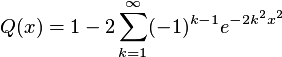
The P-value is equal to the probability of random variable with Kolmogorov-Smirnov distribution to be greater than or equal to the observed value of the KS test statistic under the null hypothesis. P-value is implemented only for Asymptotic Kolmogorov-Smirnov's distribution. c.d.f for this distribution is given by:
Data Requirements:
The Kolmogorov-Smirnov test can be performed for one or two data samples with a standard or key-type representation.
Table 19.9. Kolmogorov-Smirnov Test Settings
| Name | Description | Possible values | Default value |
|---|---|---|---|
| alpha | confidence level | real numbers from the interval (0,0.5) | 0.05 |
| distribution | distribution type | DISTRIBUTION_NORMAL, DISTRIBUTION_EXPONENTIAL, DISTRIBUTION_BETA, DISTRIBUTION_GAMMA, DISTRIBUTION_LOGISTIC | DISTRIBUTION_NORMAL |
| location | the location parameter for the selected distribution | real numbers | 0 |
| low | the lower bound parameter for the Beta distribution | real numbers | 0 |
| representation | data sample representation type | STANDARD_REPRESENTATION, SAMPLE_KEY_REPRESENTATION | STANDARD_REPRESENTATION |
| scale | the scale parameter for the selected distribution | positive real numbers | 1 |
| shape | the shape parameter for the selected distribution | positive real numbers | 1 |
| shape2 | the second shape parameter for the Beta distribution | positive real numbers | 1 |
| up | the upper bound parameter for the Beta distribution | real numbers | 1 |
Table 19.10. Kolmogorov-Smirnov Test Settings: Set Commands and View Commands
| Name | Set Command | View Command |
|---|---|---|
| alpha | settings.setAlpha(value) | settings.getAlpha() |
| distribution | settings.setDistributionType(StatisticalTestsSettings.value) | settings.getDistributionType() |
| location | settings.setLocation(value) | settings.getLocation() |
| low | settings.setLowerBound(value) | settings.getLowerBound() |
| representation | settings.setRepresentation(StatisticalTestsSettings.value) | settings.getRepresentation() |
| scale | settings.setScale(value) | settings.getScale() |
| shape | settings.setShape(value) | settings.getShape() |
| shape2 | settings.setShape2(value) | settings.getShape2() |
| up | settings.setUpperBound(value) | settings.getUpperBound() |
Example 19.8. Kolmogorov-Smirnov test
# Kolmogorov-Smirnov test example


table 'KolmogorovSmirnov':
    ks1 ks2

    1 a
    5 b
    1 b
    2 b
    5 a
    3 a
    2 b
    4 a
    1 a
    5 b
    1 b
    2 b
    5 a
    3 a
    2 b
    4 a


settings = KolmogorovSmirnovTestSettings()
settings.setAlpha(0.01)

settings.setRepresentation(StatisticalTestsSettings.SAMPLE_KEY_REPRESENTATION)
test = KolmogorovSmirnovTest(settings)

res = runStatTest(test, 'KolmogorovSmirnov', 'ks1', 'ks2')
res.printResults()
Output:
        StatTestResult:

        1) Critical value:         0.875
        2) Statistic:        0.5
        3) p-value:        Could not calculate p-Value, exact message is: Not implemented for Kolmogorov-Smirnov test.
        4) Hypothesis:        null hypotesis is accepted
This example performs the Kolmogorov-Smirnov test for two data samples from the table 'KolmogorovSmirnov" which are represented in a key-type form: the sample values are written in the first column and the second column contains keys pointing to the sample to which the given observation belongs. The first key 'a' determines the first sample and elements of the second sample are determined by the key 'b'. The null hypothesis is that both samples came from the same distribution. At the 0.01 level the null hypothesis is rejected.
This test was developed by a Dutch mathematician Nicolaas Kuiper in 1960 (see Kuiper, 1962). Kuiper's test is used to verify whether a predefined probability distribution represents the population of the data in question. In this respect it is similar to the Kolmogorov-Smirnov test. Kuiper's test, however, is equally sensitive in the tails as in the median; it is also invarian under cyclic transformations of the independent variable. Because of this, Kuiper's test is useful for testing cyclic variations (i.e. by month, day of week, etc.) in the data.
Kuiper's test is based on the empirical distribution function (EDF).
Hypothesis: One sample test
The data follows a specified distribution.
The data does not follow the specified distribution.
Two samples test:
The data follows a specified distribution.
The data does not follow the specified distribution.
The following distributions are implemented: Normal, Exponential, Logistic distribution, Beta distribution, Gamma distribution.
Test statistic:
The statistic
 for the one sided Kuiper's test is calculated according to the formulas:



where  are the
ordered distinct observations,
are the
ordered distinct observations,  is the sample size,
  is the theoretical cumulative distribution being tested and
 is the
EDF for the sample.
is the
EDF for the sample.
The asymptotic statistic value is calculated as

The statistic
 for the two sided Kuiper's test is calculated according to the formulas:



where
 is the first sample size,
 is the second sample size,
 ,
and
,
and  and
and  are the EDF-s for the firs and second sample respectively.
The asymptotic statistic value for the two sided test is calculated as
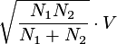

The null hypothesis is rejected if the value of the Kuipr's test statistic calculated for the given sample is greater than the corresponding critical value of the distribution of the Kuiper's test statistic. This distribution depends on sample size and confidence level.
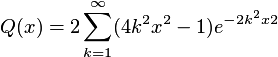
The P-value is equal to the probability of a random variable with Kuiper's distribution to be greater or equal to the observed value of Kuiper's test statistic under the null hypothesis. The P-value is implemented only for the asymptotic Kuiper's distribution. The CDF for distribution is given by the formula
.
Data requirements:
Kuiper's test can be performed for one or two data samples with a standard or key-type representation
Table 19.11. Kuiper's test settings
| Name | Description | Possible values | Default value |
|---|---|---|---|
| alpha | confidence level | real numbers from the interval (0,0.5) | 0.05 |
| distribution | distribution type | DISTRIBUTION_NORMAL, DISTRIBUTION_EXPONENTIAL, DISTRIBUTION_BETA, DISTRIBUTION_GAMMA, DISTRIBUTION_LOGISTIC | DISTRIBUTION_NORMAL |
| location | the location parameter for the selected distribution | real numbers | 0 |
| low | the lower bound parameter for the Beta distribution | real numbers | 0 |
| representation | data sample representation type | STANDARD_REPRESENTATION, SAMPLE_KEY_REPRESENTATION | STANDARD_REPRESENTATION |
| scale | the scale parameter for the selected distribution | positive real numbers | 1 |
| shape | the shape parameter for the selected distribution | positive real numbers | 1 |
| shape2 | the second shape parameter for the Beta distribution | positive real numbers | 1 |
| up | the upper bound parameter for the Beta distribution | real numbers | 1 |
Table 19.12. Kuiper's test settings: set commands and view commands
| Name | Set Command | View Command |
|---|---|---|
| alpha | settings.setAlpha(value) | settings.getAlpha() |
| distribution | settings.setDistributionType(StatisticalTestsSettings.value) | settings.getDistributionType() |
| location | settings.setLocation(value) | settings.getLocation() |
| low | settings.setLowerBound(value) | settings.getLowerBound() |
| representation | settings.setRepresentation(StatisticalTestsSettings.value) | settings.getRepresentation() |
| scale | settings.setScale(value) | settings.getScale() |
| shape | settings.setShape(value) | settings.getShape() |
| shape2 | settings.setShape2(value) | settings.getShape2() |
| up | settings.setUpperBound(value) | settings.getUpperBound() |
Levene's test (Levene 1960) is used to check whether two samples have equal variances. The occurrence of equal variances across samples is called the homogeneity of variance . Some statistical tests, for example the analysis of variance, assume that variances are equal across groups of samples. Levene's test can be used to verify that assumption. The original variant of Levene's test uses absolute deviations from the sample mean. Brown and Forsythe in 1974 proposed using the absolute deviations from the median or from the trimmed mean in addition to the usual mean value.
There are three variants of Levene's test: mean-based, median-based and 10%-trimmed mean based. In each case the absolute deviations from the above values are used.
The originally proposed test used mean values of the sample. Brown and Forsythe, 1974 performed Monte Carlo simulations and showed that using the trimmed mean performed best when the underlying data followed a Cauchy distribution and the median performed best when the underlying data followed a chi-square distribution. Using the mean provided the best power for symmetric distributions without heavy tails. Although the optimal choice of the test variant depends on the underlying distribution, the variant based on the median is recommended as the choice that provides good robustness against many types of non-normal data while retaining good power. Knowledge of the underlying distribution of the data may suggest using one of the other variants.
Hypothesis:
The two data samples have equal variances.
The two data samples do not have equal variances.
Test Statistic:
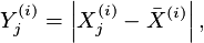
Levene's test statistic is calculated as follows:

with
 calculated as follows:
where
 denotes the mean value of the sample i.
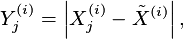
where
 denotes the median value of the sample i.
3. For the 10%-trimmed mean based test:
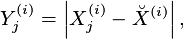
where
 denotes the 10%-trimmed mean of the sample i.
In the above  denotes the in-sample (over j)
mean value of
denotes the in-sample (over j)
mean value of  and
and  denotes the overall mean of
 .
.
These three choices for calculating  determine the robustness and power of
Levene's test.
determine the robustness and power of
Levene's test.

The null hypothesis is rejected if the calculated value
 of the test statistic is greater than the
corresponding critical value:
of the test statistic is greater than the
corresponding critical value:

where  is the upper critical value of an
F-distribution with
is the upper critical value of an
F-distribution with  degrees of freedom.
The P-value is equal to probability of a random variable with an
F-distribution with  degrees of freedom to be
greater than or equal to the observed value of the Levene's test
statistic under the null hypothesis.
degrees of freedom to be
greater than or equal to the observed value of the Levene's test
statistic under the null hypothesis.
Data Requirements:
Levene's test is performed for two numerical data samples with a standard or key-type representation.
Table 19.13. Levene's Test Settings
| Name | Description | Possible values | Default value |
|---|---|---|---|
| alpha | confidence level | real numbers from the interval (0,0.5) | 0.05 |
| choice | the variant of Levene's test to be used | MEAN_BASED, MEDIAN_BASED, TRIMMED_MEAN_BASED | MEAN_BASED |
| representation | data sample representation type | STANDARD_REPRESENTATION, SAMPLE_KEY_REPRESENTATION | STANDARD_REPRESENTATION |
Table 19.14. Levene's Test Settings: Set Commands and View Commands
| Name | Set Command | View Command |
|---|---|---|
| alpha | settings.setAlpha(value) | settings.getAlpha() |
| choice | settings.setChoice(StatisticalTestsSettings.value) | settings.getChoice() |
| representation | settings.setRepresentation(StatisticalTestsSettings.value) | settings.getRepresentation() |
Example 19.9. Levene's test
# Levene test example


table 'Levene':
    l1 l2

    1 2
    3 3
    1 4
    2 2
    3 3
    3 2
    2 3
    3 2
    1 4
    2 1
    1 2
    2 3
    2 4
    3 2
    2 2
    4 2

settings = LeveneTestSettings()
settings.setAlpha(0.2)
test = LeveneTest(settings)

res = runStatTest(test, 'Levene', 'l1', 'l2')
res.printResults()
Output:
        StatTestResult:

        1) Critical value:         0.06533410259213834
        2) Statistic:        0.020104244229337303
        3) p-value:        0.8881942426257567
        4) Hypothesis:        null hypotesis is accepted
The above example applies Levene's test to check whether the two data samples come from the populations with equal variances. At 0.2 level of confidence the null hypothesis about equal variances is accepted.
The Mann-Whitney test is a non-parametric (distribution-free) test used to compare two independent data samples.
The Mann-Whitney test is an alternative to the independent samples t-test, used when the assumption of normality or equality of variance is not met. This, like many non-parametric tests, uses the ranks of the data rather than their raw values to calculate the statistic. Since this test does not make any assumption about the distribution, it is not as powerful as the t-test.
The Mann-Whitney test is also called the Mann-Whitney rank sum test or rank sum test. Even though this test is commonly called the Mann-Whitney test, it was in fact developed by Wilcoxon and sometimes is also called the Wilcoxon test.
The t-test is the standard method for testing whether the population means for two non-paired samples are equal. If the populations are non-normal, particularly for small samples, then the t-test may not be valid. The Mann-Whitney test is an alternative that can be applied when the distributional assumptions are suspect. However, it is not as powerful as the t-test when the distributional assumptions are in fact valid. To perform the Mann-Whitney test the first step is to rank the combined samples. Then the sum of the ranks for sample one and the sum of the ranks for sample two are computed and these ranks are used for the calculation of the test statistic. For more details see for example Lehmann 1975.
Hypothesis:
The two data samples have equal means.

Two-sided test: The two populations do not have equal means.
Left-sided test: The mean value of the first population is less than the mean value of the second population.
Right-sided test: The mean value of the first population is greater than the mean value of the second population.
Test Statistic:
To perform the Mann-Whitney test the first step is to rank the
combined samples. Then the sum of the ranks for sample one (
 ) is computed. The following statistics
are calculated:
) is computed. The following statistics
are calculated:

where  and
and  are the sample sizes.
Two-sided test :
If the sample sizes are equal, the Mann-Whitney test statistic
 is the minimum of the two values:

Left-sided test :

Right-sided test :

For sufficiently large samples (sample size greater than 20), the following normal approximation is used:
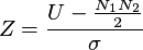
where

For small sample sizes it is necessary to use special tables of critical values.

The null hypothesis is rejected if:
Two-sided
test
: the calculated value of the test statistic
 is greater than the critical value

One-sided
test
s: the calculated value of the test
statistic  is greater than the critical value
 , where
  is the standard normal distribution
quantile.
is the standard normal distribution
quantile.
The P-value is equal to the probability of a random variable with a standard normal distribution to be greater or equal to the observed value of the Mann-Whitney test statistic under the null hypothesis.
Data Requirements:
The Mann-Whitney test is performed for two numerical data samples with a standard or key-type representation.
Table 19.15. Mann-Whitney Test Settings
| Name | Description | Possible values | Default value |
|---|---|---|---|
| alpha | confidence level | real numbers from the interval (0,0.5) | 0.05 |
| representation | data sample representation type | STANDARD_REPRESENTATION, SAMPLE_KEY_REPRESENTATION | STANDARD_REPRESENTATION |
| side | the type of the test | TWO_SIDED, LEFT_SIDED, RIGHT_SIDED | TWO_SIDED |
Table 19.16. Mann-Whitney Test Settings: Set Commands and View Commands
| Name | Set Command | View Command |
|---|---|---|
| alpha | settings.setAlpha(value) | settings.getAlpha() |
| representation | settings.setRepresentation(StatisticalTestsSettings.value) | settings.getRepresentation() |
| side | settings.setSide(StatisticalTestsSettings.value) | settings.getSide() |
Example 19.10. Mann-Whitney test
# Mann-Whitney test example


table 'MannWhitney':
    mw1 mw2

    43   99
    97   98
    102  94
    101  86
    12   56
    97   103
    103  99
    104  89
    109  102
    59   104
    90   103
    98   96
    86   67
    92   90
    95   105
    101  79
    89   87

settings = MannWhitneyTestSettings()
test = MannWhitneyTest(settings)

res = runStatTest(test, 'MannWhitney', 'mw1', 'mw2')
res.printResults()
Output:
        StatTestResult:

        1) Critical value:         1.9599639845400536
        2) Statistic:        -0.08610882996604705
        3) p-value:        0.9313798362985003
        4) Hypothesis:        null hypotesis is accepted
The above example performs the Mann-Whitney test for the data samples 'mw1' and 'mw2' and checks whether these samples come from populations with equal means and at the default confidence level of 0.05 the test proves this assumption.
Pearson's test is a t-test for the significance of Pearson's product moment correlation coefficient. Pearson's product moment correlation coefficient is a parametric measure of linear correlation between two variables. It measures both the strength and direction of a linear relationship. If there is no linear predictability between the two variables, the correlation is 0. If the two variables are normal with zero correlation, the two variables are independent. However, correlation does not imply causality because, in some cases, an underlying causal relationship may not exist.
Pearson's product moment correlation is an example of a correlation coefficient. It is a measure of the linear association between two variables that have been measured on interval or ratio scales. However, one should remember that it can be misleadingly small when there is a relationship between the variables but it is not a linear one.
For two variables  and
and  Pearson's correlation coefficient is
calculated as:
Pearson's correlation coefficient is
calculated as:
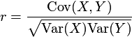
For two paired samples Pearson's sample correlation coefficient is calculated as:
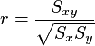
where
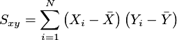
and  is the sample size.
Pearson's sample correlation coefficient has the following properties:
it only measures the strength of a linear relationship,
it is always between -1 and 1 inclusive: -1 means a perfect negative linear correlation and +1 means a perfect positive linear correlation between the variables,
it has the same sign as the slope of the regression (best fit) line,
it does not change if the scale of either variable is changed,
it has a Student t-distribution.
Hypothesis:
The two variables are not correlated.

Two-sided test: the two variables are correlated.
Left-sided test: the two variables are negatively correlated.
Right-sided test: the two variables are positively correlated.
Note
The one-sided test can be misleading if two-sided test has rejected the null hypothesis. The correct result will give the one-sided test which also have rejected the null hypothesis.
Test Statistic:
The Pearson's Test for the correlation coefficient is based on the statistic:
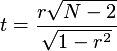
where
 is a sample Pearson's product moment
correlation and
is a sample Pearson's product moment
correlation and  is the sample size, which has the Student
t-distribution with
is the sample size, which has the Student
t-distribution with  degrees of freedom.

The null hypothesis is rejected if:
Two-sided test : the calculated absolute value of the test statistic is greater than the corresponding critical value:

and
Left-sided test : the calculated value of the test statistic is less than the corresponding critical value

Right-sided test : the calculated value of the test statistic is greater than the corresponding critical value

where  are the upper quantiles of the
Student t-distribution with
are the upper quantiles of the
Student t-distribution with  degrees of freedom.
The P-value is equal to the probability of a random variable
with a Student t-distribution with  degrees of freedom to be greater or equal
to the calculated value of the test statistic under the null
hypothesis.
degrees of freedom to be greater or equal
to the calculated value of the test statistic under the null
hypothesis.
Data Requirements:
The Pearson's test is performed for two data samples of equal length with standard or key-type representation.
Table 19.17. Pearson's Test Settings
| Name | Description | Possible values | Default values |
|---|---|---|---|
| alpha | confidence level | real numbers from the interval (0,0.5) | 0.05 |
| representation | data sample representation type | STANDARD_REPRESENTATION, SAMPLE_KEY_REPRESENTATION | STANDARD_REPRESENTATION |
| side | the type of the test | TWO_SIDED, LEFT_SIDED, RIGHT_SIDED | TWO_SIDED |
Table 19.18. Pearson's Test Settings: Set Commands and View Commands
| Name | Set Command | View Command |
|---|---|---|
| alpha | settings.setAlpha(value) | settings.getAlpha() |
| representation | settings.setRepresentation(StatisticalTestsSettings.value) | settings.getRepresentation() |
| side | settings.setSide(StatisticalTestsSettings.value) | settings.getSide() |
Example 19.11. Pearson's test
# Pearson's test example

table 'Pearson':
    p1 p2

    1    0.99
    0.97 0.98
    1    0.99
    1.1  1
    1.2  1.1
    1.2  1.3
    1.3  1.2
    1.4  1.23
    1.4  1.25
    1.5  1.4
    1.4  1.3
    2.3  1.6
    2.4  1.67
    3.2  2
    3.5  2.2
    4.2  2.7

settings = PearsonTestSettings()
test = PearsonTest(settings)

res = runStatTest(test, 'Pearson', 'p1', 'p2')
res.printResults()
Output:
        StatTestResult:

        1) Critical value:         2.144786686484972
        2) Statistic:        22.99605651079155
        3) p-value:        1.6084911180769268E-12
        4) Hypothesis:        null hypotesis is rejected
The above example tested the hypothesis about no correlation between the data samples 'p1' and 'p2' and rejected this hypothesis. It means that there is a strong correlation between these two variables at 0.05 level of confidence.
Test of proprtions is used to determine whether the proportion of a given feature in a population is equal to a pre-defined value (one sample test) or whether the proprtions of a given feature in two populations are equal (two sample test)
Test of proprtions van be applied to numerical variables which assume two distinct values.
It is assumed that the investigated value has a Bernoulli distribution with the parameter
 . Let
. Let
 denote
the actual proprtion of the category in the sample, i.e.
denote
the actual proprtion of the category in the sample, i.e.
 ,
where
,
where  is the sample size and
  is the number of occurences of the given category.
For the test results to be reliable the condition that
 and
and  should be satisfied.
Hypothesis:


Two-sided test:

Right-sided test:

Left-sided test:

Test statistic:
The statistic for the one sample test of proprtions is calculated as
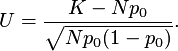
Under the null hypothesis this statistic has the  normal distribution.

The null hypothesis is rejected, if:
Two-sided test:
Right-sided test:
Left-sided test:
where
is the inverse of the distribution function for the
distribution.



P-value: Under the null hypothesis the P-value is equal to the
probability that a random variable with  distribution is greater or equal than the calculated
value of the test statistic. For the one-sided test the null hypothesis is rejected
if p-value is less than
distribution is greater or equal than the calculated
value of the test statistic. For the one-sided test the null hypothesis is rejected
if p-value is less than  . For the two sided test the null hypothesis
is rejected if p-value is less than
. For the two sided test the null hypothesis
is rejected if p-value is less than  .
.
Data requirements: The one sample test of proprtions can be performed on a numerical data sample which assumes at most two different values. Both standard and key-type representations are accepted.
It is assumed that the investigated value has a Bernoulli distribution with the parameter
 in the
first sample and
in the
first sample and  in the second sample. Let
  and
and  denote the counts of the first and second sample respectively and
 and
and
 the counts
of occurences of the investigated categories in the first and second sample respectively.
the counts
of occurences of the investigated categories in the first and second sample respectively.
For the test results to be reliable the condition that  should be satisfied.
Hypothesis:


Two-sided test:

Right-sided test:

Left-sided test:

Test statistic:
The statistic for the one sample test of proprtions is calculated as
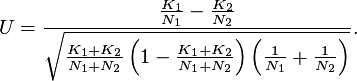
Under the null hypothesis this statistic has the  normal distribution.

The null hypothesis is rejected, if:
Two-sided test:
Right-sided test:
Left-sided test:
where
is the inverse of the distribution function for the
distribution.



P-value: Under the null hypothesis the P-value is equal to the
probability that a random variable with  distribution is greater or equal than the calculated
value of the test statistic. For the one-sided test the null hypothesis is rejected
if p-value is less than
distribution is greater or equal than the calculated
value of the test statistic. For the one-sided test the null hypothesis is rejected
if p-value is less than  . For the two sided test the null hypothesis
is rejected if p-value is less than
. For the two sided test the null hypothesis
is rejected if p-value is less than  .
.
Data requirements: The two sample test of proprtions can be performed on a pair of numerical data samples (variables) which assume at most two different values. Both standard and key-type representations are accepted.
Table 19.19. Test of proportions settings
| Name | Description | Possible values | Default value |
|---|---|---|---|
| alpha | confidence level | real numbers from the interval (0,0.5) | 0.05 |
| representation | data sample representation type | STANDARD_REPRESENTATION, SAMPLE_KEY_REPRESENTATION | STANDARD_REPRESENTATION |
| side | the type of the test | TWO_SIDED, LEFT_SIDED, RIGHT_SIDED | TWO_SIDED |
| distinctValue | the value the proportion of which is being tested | real numbers | 0.0 |
| expectedProportion | for the one sample test, the parameter of the Bernoulli distribution against which the sample is being tested. | real numbers from the interval [0, 1] |
Table 19.20. Test of proportions settings: Set Commands and View Commands
| Name | Set Command | View Command |
|---|---|---|
| alpha | settings.setAlpha(value) | settings.getAlpha() |
| representation | settings.setRepresentation(StatisticalTestsSettings.value) | settings.getRepresentation() |
| side | settings.setSide(StatisticalTestsSettings.value) | settings.getSide() |
| distinctValue | settings.setDistinctValue(value) | settings.getDistinctValue() |
| expectedProportion | settings.setExpectedProportion(value) | settings.getExpectedProportion() |
This example tests the proportion of good debtors Class in the german_credit dataset. Note that the categorical variable 'Class' needs to be transformed to a numerical binary variable before the test can be performed.
Example 19.12. One sample test of proportions
# prepare data sample for testing: add a binary
# numerical variable 'Class_num' based on the
# categorical variable "Class".
trans 'german_credit_1' <- 'german_credit':
    if Class == 'good':
        Class_num = 1
    else:
        Class_num = 0

# prepare ProportionTestSettings and the test object
settings = ProportionTestSettings()
settings.setAlpha(0.05)
settings.setExpectedProportion(0.75)
settings.setDistinctValue(1)
settings.setSide(StatisticalTestsSettings.RIGHT_SIDED)

test = ProportionTest(settings)

# execute the test and print the results
res = runStatTest(test, 'german_credit_1', 'Class_num')
res.printResults()
Output:
        StatTestResult:

        1) Critical value:         1.6448536269514715
        2) Statistic:        -3.6514837167011107
        3) p-value:        0.9998696351720902
        4) Hypothesis:        null hypotesis is rejected
In 1710 Dr. John Arbuthnott published a paper in which he tried to prove God's existence. The title of the paper was "An Argument for Divine Providence, Taken from the Constant Regularity Observ'd in the Birth of Both Sexes". It is not clear whether Dr. Arbuthnott has proven 'Divine Providence' with his arguments, but it is commonly believed that the scientific method represented in that article was the beginning of the oldest type of statistical tests, namely the Sign Test.
The Sign test is specifically designed for testing hypotheses about the median of any continuous population. It was first suggested for use in speech recognition benchmark tests. The median is a measure of the location (center) of the distribution, therefore the Sign test is sometimes referred to as the test for location).
The Sign test is generally less powerful than the Mann-Whitney (Wilcoxon) test. It is, however, simple and easy to use. For small samples the level of significance can be estimated without the help of a calculator or table. If the Sign test indicates a significant difference and another test does not, it is necessary to seriously consider whether the other test is valid.
The Sign test is used to test the hypothesis about the median of a population.
The sign test uses the following statistic:

Note that the value of this statistic depends only on the sign
(positive or negative) of the difference between sample values and the
tested median value. That is, the statistic simply counts the number
of positive (or negative) signs among the above differences. If
 is too large, the null hypothesis will be
rejected in favor of the alternative hypothesis. Since the
observations are independent the properties of a binomial distribution
are satisfied and therefore the statistic
is too large, the null hypothesis will be
rejected in favor of the alternative hypothesis. Since the
observations are independent the properties of a binomial distribution
are satisfied and therefore the statistic  has a binomial distribution with the
parameters {the number of sample elements} and p = 0.5. For samples
with more than 10 elements the normal approximation for binomial
distribution can be used since it performs reasonably well even for
sample size equal to 10. For more details see for example Conover
1980, Hollander and Wolfe 1973.
has a binomial distribution with the
parameters {the number of sample elements} and p = 0.5. For samples
with more than 10 elements the normal approximation for binomial
distribution can be used since it performs reasonably well even for
sample size equal to 10. For more details see for example Conover
1980, Hollander and Wolfe 1973.
Hypothesis:
The population median is equal to


Two-sided test: the population median is not equal to

Left-sided test: the population median is less than

Right-sided test: the population median is greater than

Test Statistic:
For a sample  ,
,
 the Sign test
statistic is calculated according to the following RULE:
the Sign test
statistic is calculated according to the following RULE:
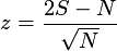
 is calculated for the two-sided test
as
is calculated for the two-sided test
as

where

(here
 denotes the cardinality of the set
 )
)
For the left-side test 
and for the right-sided test  , where
  is the tested median value.

The null hypothesis is rejected if:
Two-sided test : the absolute value of the calculated test statistic is greater than the corresponding critical value:

Left-sided test : the calculated test statistic is less than the corresponding critical value:

Right-sided test : the calculated test statistic is greater than the corresponding critical value:

Here  denotes the upper percentile of the
standard normal distribution.
denotes the upper percentile of the
standard normal distribution.
The P-value is equal to the probability of a random variable with a standard normal distribution to be greater than or equal to the observed value of the Sign test statistic under the null hypothesis.
Data Requirements:
The Sign test can be performed on two numerical data samples with a standard or key-type representation.
Table 19.21. Sign Test Settings
| Name | Description | Possible values | Default value |
|---|---|---|---|
| alpha | confidence level | real numbers from the interval (0,0.5) | 0.05 |
| mZero | the mZero value of the population median for the null hypothesis | real numbers | 0 |
| representation | data sample representation type | STANDARD_REPRESENTATION, SAMPLE_KEY_REPRESENTATION | STANDARD_REPRESENTATION |
| side | the type of the test | TWO_SIDED, LEFT_SIDED, RIGHT_SIDED | TWO_SIDED |
Table 19.22. Sign Test Settings: Set Commands and View Commands
| Name | Set Command | View Command |
|---|---|---|
| alpha | settings.setAlpha(value) | settings.getAlpha() |
| mZero | settings.setMZero(value) | settings.getMZero() |
| representation | settings.setRepresentation(StatisticalTestsSettings.value) | settings.getRepresentation() |
| side | settings.setSide(StatisticalTestsSettings.value) | settings.getSide() |
Example 19.13. Sign test
#  Sign test example

table 'Sign':
    s

    739
    978
    1094
    1086
    856
    803
    399
    489
    902
    904
    903
    996
    867
    990
    955
    1079
    897

settings = SignTestSettings()
settings.setAlpha(0.1)
settings.setMZero(900)

test = SignTest(settings)

res = runStatTest(test, 'Sign', 's')
res.printResults()
Output:
        StatTestResult:

        1) Critical value:         1.6448536269514715
        2) Statistic:        0.48507125007266594
        3) p-value:        0.6276257639467913
        4) Hypothesis:        null hypotesis is accepted
The above example performs the Sign test to check whether the sample data 's' came from a population with a median value of 900, and at the confidence level of 0.1 this hypothesis is accepted.
Different non-parametric statistics have been invented to measure and test for correlation between two random variables. Spearman's rank (rank-order) correlation coefficient is one example of a correlation coefficient. Usually it is calculated when for some reasons the actual values or variables are not given, but only a rank order is assigned to the instance of each variable. Spearman's rank-order correlation coefficient may also be a better measure of dependence between the two variables when the relationship between them is non-linear. Spearman's rank-order correlation is a nonparametric measure of dependency between two paired samples and is based on the ranks of the paired data.
Spearman's rank-order correlation is a nonparametric measure of dependency between two paired samples and is based on the ranks of the paired data. Spearman's test is used to check the significance of rank correlation coefficient.
For  pairs of observations
  Spearman's rank-order correlation
is calculated as
Spearman's rank-order correlation
is calculated as
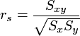
where
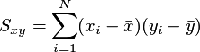
and

Here  and
and  are the ranks of pairs of observations.
When there are no ties the above formula is reduced to
are the ranks of pairs of observations.
When there are no ties the above formula is reduced to
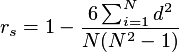
where  is the difference between the
pair ranks.
is the difference between the
pair ranks.
Hypothesis:
The data are not correlated

Two-sided test: the data are correlated;
Left-sided test: the data are negatively correlated;
Right-sided test: the data are positively correlated.
Note
The one-sided test can be misleading if the two-sided test rejected the null hypothesis. The correct result will give the one-sided test which have also rejected the null hypothesis.
Test Statistic: Spearman's test statistic is defined as
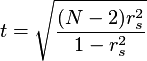
The statistic has a Student t-distribution with  degrees of freedom.

The null hypothesis is rejected if:
Two-sided
test
: the absolute value of the test statistic
is greater than the critical value; the critical value is equal to
 percentile of t-Student
distribution with
percentile of t-Student
distribution with  degrees of freedom;
Left-sided test : the value of the test statistic is less than the negative critical value;
Right-sided test : the value of the test statistic is greater than the critical value.
The critical value for the one-sided alternatives is equal to
 percentile of a Student
t-distribution with
percentile of a Student
t-distribution with  degrees of freedom.
The P-value is equal to the probability that a random variable
with a Student t-distribution with  degrees of freedom will be greater than
or equal to the calculated value of the test statistic.
degrees of freedom will be greater than
or equal to the calculated value of the test statistic.
Data Requirements:
Spearman's correlation test can be performed for two numerical data samples of equal length with a standard or key-type representation.
Table 19.23. Spearman's Test Settings
| Name | Description | Possible values | Default value |
|---|---|---|---|
| alpha | confidence level | real numbers from the interval (0,0.5) | 0.05 |
| representation | data sample representation type | STANDARD_REPRESENTATION, SAMPLE_KEY_REPRESENTATION | STANDARD_REPRESENTATION |
| side | the type of the test | TWO_SIDED, LEFT_SIDED, RIGHT_SIDED | TWO_SIDED |
Table 19.24. Spearman's Test Settings: Set Commands and View Commands
| Name | Set Command | View Command |
|---|---|---|
| alpha | settings.setAlpha(value) | settings.getAlpha() |
| representation | settings.setRepresentation(StatisticalTestsSettings.value) | settings.getRepresentation() |
| side | settings.setSide(StatisticalTestsSettings.value) | settings.getSide() |
Example 19.14. Spearman's test
#  Spearman's Test example

table 'Spearman':
    p1 p2

    1    0.99
    0.97 0.98
    1    0.99
    1.1  1
    1.2  1.1
    1.2  1.3
    1.3  1.2
    1.4  1.23
    1.4  1.25
    1.5  1.4
    1.4  1.3
    2.3  1.6
    2.4  1.67
    3.2  2
    3.5  2.2
    4.2  2.7

settings = SpearmanTestSettings()
settings.setSide(StatisticalTestsSettings.RIGHT_SIDED)
test = SpearmanTest(settings)

res = runStatTest(test, 'Spearman', 'p1', 'p2')
res.printResults()
Output:
        StatTestResult:

        1) Critical value:         1.7613101352742437
        2) Statistic:        14.138496161073997
        3) p-value:        5.551056281305478E-10
        4) Hypothesis:        null hypotesis is rejected
The above example performs Spearman's correlation test for the same data as the example for Pearson's correlation test, which checked if the two samples were not correlated or positively correlated. Indeed, these data samples are positively correlated.
Student's t-test is used to determine whether there is a significant difference between the means of two populations (two-samples test) or whether the population mean differs significantly from a predetermined mean value.
It is assumed that the data sets are drawn from normally distributed populations and for the two-samples test it can be additionally required that these populations have equal variances.
What if the conditions for the validity of Student's t-test are not valid? In this situation the best approach is to transform the data to a scale in which the conditions are satisfied. This will almost always involve a logarithmic transformation. Sometimes a square root, inverse, or inverse square root might be used. For proportions, arcsin(sqrt(p)) or log(p/(1-p)) might be used. If no satisfactory transformation can be found, a nonparametric test such as the median test or the Mann-Whitney test might be used.
Note: both equal and unequal variance versions of the test are implemented for the two-samples unpaired test and an equal variance version of the test is implemented for the two-samples paired test.
"Student" was the pseudonym of William Sealey Gosset (1876-1937) an Irish Guinness brewery worker. In 1908 he published a paper showing that a certain probability distribution, now called the Student distribution or the t-distribution, arises in the problem of estimating the mean of a normally distributed population when the sample size is small. The basis of the t-test would be known as 'Gosset's t-distribution' if it were not for contractual obligations that prevented W.S. Gosset from taking credit for its development. Because of some problems with another worker in the past (he published the company's secrets) the brewery had prohibited workers to publish anything. Guinness agreed to let Gosset publish his statistical research provided that he used a pseudonym (he used "A Student") and that none of the company data would appear in the publication. So Gosset used measurements of the heights and left middle finger lengths of criminals in the local prison to work out the t-distribution empirically.
Student's t test for independent samples is used to determine whether two samples were drawn from populations with different means or whether the population mean is different from some predefined value. Student's t-test, often known simply as the t-test, is one of the most commonly used statistical tests. It comes in two versions: the paired t-test and the unpaired t-test. Both types are used to test the hypothesis that the mean values differ between the two populations, but the paired test is particularly useful when each observation in one sample corresponds to a matching observation in the other sample. The unpaired t-test is a more general technique that can be used to test whether the mean value differs between the two populations and does not require that the two samples be paired in any way or even have equal sizes.
For two unpaired samples if both of them are large enough, the separate or unequal variance version of the Student's t-test has many attractive features. The denominator of the test statistic correctly estimates the standard deviation of the numerator, while the Central Limit Theorem guarantees the validity of the test even if the populations are non-normal. "Large enough" sample sizes can be as small as 30 per sample if the two populations are nearly normally distributed. The more the populations depart from normality the larger the sample size needed for the Central Limit Theorem to support the test result. Note that 100 observations is often a quite sufficient sample size. For small and moderate sample sizes, the equal variances version of the test provides an exact test of the equality of the two population means. In this case the validity of the test demands that the samples be drawn from normally distributed populations with equal variances.
Hypothesis:
One-sample test :
the population mean is equal to
.

Two-sided test: the population mean is not equal to

Left-sided test: the population mean is less than

Right-sided test: the population median is greater than

Two-samples unpaired test :
The two populations have equal means.

Two-sided test: the two populations do not have equal means;
Left-sided test: the mean value of the first population is less than the mean value of the second population;
Right-sided test: the mean value of the first population is greater than the mean value of the second population.
Two-samples paired test :
The mean difference between the two populations is equal to
.

Two-sided test: the mean difference between the two populations is not equal to
;
Left-sided test: the mean difference between the two populations is less than
;
Right-sided test: The mean difference between the two populations is greater than
.
Test Statistic:
For
a sample  Student's t-test statistic is calculated as:
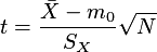
where  is the sample mean value and
 is the sample standard deviation,
 is the sample size.
For
two paired
samples
 the t-test statistic
is calculated as:
the t-test statistic
is calculated as:
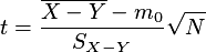
where  is the mean value of the
differences
is the mean value of the
differences  and
and
 is the standard deviation of these
differences,
is the standard deviation of these
differences,  is the sample size.
For
two unpaired samples
 under
the unequal variances assumption the t-test statistic is calculated as:
under
the unequal variances assumption the t-test statistic is calculated as:
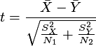
where  and
and  are the mean values of the samples
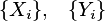 ,
,
 and
and  are the sample standard deviations,
 and
and 
are the sample sizes.
For
two unpaired
samples
 under
equal variances assumption the t-test statistic is calculated as:
under
equal variances assumption the t-test statistic is calculated as:
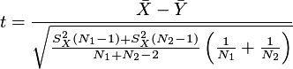
where  and
and  are the mean values of the samples
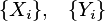 ,
,
 and
and  are the sample standard deviations,
  and
and  are the sample sizes.

The null hypothesis is rejected if:
Two-sided
test
: the absolute value of the test statistic
is greater than the critical value; the critical value is equal to:
 percentile of Student's
t-distribution with
percentile of Student's
t-distribution with  degrees of freedom;
Left-sided test : the value of the test statistic is less than the negative critical value;
Right-sided test : the value of the test statistic is greater than the critical value.
The critical value for the one-sided alternatives is equal to
 percentile of Student's
t-distribution with
percentile of Student's
t-distribution with  degrees of freedom.
Degrees of freedom are defined as
for the one-sample test and for the two-samples paired test:
,
for the two-samples unpaired test under the equal variances assumption:

for the two-samples unpaired test under the unequal variances assumption:
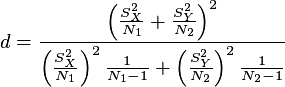
The P-value is equal to the probability of a random variable
with a Student's t-distribution with  degrees of freedom to be greater or equal
to the calculated absolute value of the test statistic under the null
hypothesis.
degrees of freedom to be greater or equal
to the calculated absolute value of the test statistic under the null
hypothesis.
Data Requirements:
The Student's t-test can be performed for one or two numerical data samples with a standard or sample-key representation.
Table 19.25. Student's T-test Settings
| Name | Description | Values | Default |
|---|---|---|---|
| alpha | confidence level | real numbers from the interval (0,0.5) | 0.05 |
| meanZero | the value of the population mean to be tested | real number | 0 |
| pair | the type of StudentTTest test for two samples (0 for non-paired and 1 for paired test) | NON_PAIRED, PAIRED | NON_PAIRED |
| representation | data sample representation type | STANDARD_REPRESENTATION, SAMPLE_KEY_REPRESENTATION | STANDARD_REPRESENTATION |
| side | the type of the test | TWO_SIDED, LEFT_SIDED, RIGHT_SIDED | TWO_SIDED |
| varEqual | determines whether the equal or unequal variances assumption should be used | EQUAL_VARIANCES, UNEQUAL_VARIANCES | EQUAL_VARIANCES |
Table 19.26. Student's T-test Settings: Set Commands and View Commands
| Name | Set Command | View Command |
|---|---|---|
| alpha | settings.setAlpha(value) | settings.getAlpha() |
| meanZero | settings.setMeanZero(value) | settings.getMeanZero() |
| pair | settings.setPair(StatisticalTestsSettings.value) | settings.getPair() |
| representation | settings.setRepresentation(StatisticalTestsSettings.value) | settings.getRepresentation() |
| side | settings.setSide(StatisticalTestsSettings.value) | settings.getSide() |
| varEqual | settings.setVarEqual(StatisticalTestsSettings.value) | settings.getVarEqual() |
Example 19.15. Student's test
# Student t-test example


table 'Student':
    s

    2.1
    3.1
    1.5
    1.1
    1.2
    1.2
    1.3
    1.4
    1.4
    1.5
    1.4
    2.4
    3.2
    3.5
    4.2

settings = StudentTTestSettings()
settings.setMeanZero(2)
test = StudentTTest(settings)

res = runStatTest(test, 'Student', 's')
res.printResults()
Output:
        StatTestResult:

        1) Critical value:         2.144786686484972
        2) Statistic:        0.12885424152806213
        3) p-value:        0.8993058080007479
        4) Hypothesis:        null hypotesis is accepted
The above example applies Student's t-test to check if the data sample 's' came from the distribution with the mean value equal to 2. The test showed that this hypothesis can be accepted at the default confidence level.
[3] (1974) Robust Tests for Equality of Variances, Journal of the American Statistical Association, 364 - 367.
[7] (1962) Tests concerning random points on a circle , Proceedings of the Koninklijke Nederlandse Akademie van Wetenschappen, Series A , 38-47.
[9] (1960) In: Contributions to Probability and Statistics: Essays in Honor of Harold Hotelling , , Stanford University Press, Palo Alto.
[10] (1961) Distribution of Anderson-Darling Statistic , Annals of Mathematical Statistics, 1118-1124.
[12] (1974) EDF Statistics for Goodness of Fit and Some Comparisons , Journal of the American Statistical Association, 730-737.
[13] (1976) Asymptotic Results for Goodness-of-Fit Statistics with Unknown Parameters , Annals of Statistics, 357-369.