Table of Contents
This section discuses the methods for the calculation of various statistical characteristics of data sets in AdvancedMiner.
The freq, chiSquare and Pearson procedures are capable of sending output to MS Office Excel or OpenOffice Spreadsheet, provided the appropriate office suite connection is set in AdvancedMiner options dialog. Refer to the Integration with common office suiteschapter for more details. It is also possible to display the resulting spreadsheet intrnally in AdvancedMiner, by selecting Internal components in the AdvancedMiner Options dialog.
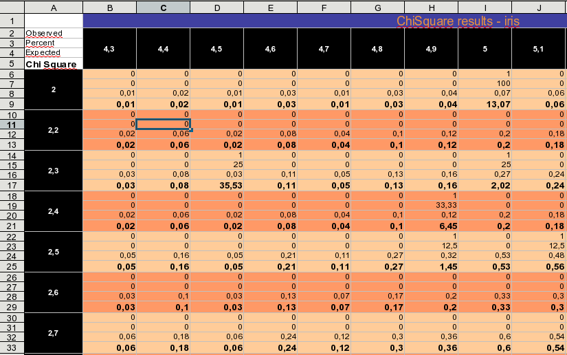
The chiSquare function calculates the value of the Chi-square statistic for the dependent and independent variables. Adittionally, the total number of appearances, percentages in the total number and the expected number of appearances are calculated.
Rows with NULL values are omitted.
An example chiSquare output is shown below
Syntax:
chiSquare(alias.table, independent, dependent, silent = 0|1)
alias - an alias pointing to a database, if omitted, the default alias is used.
table - the name of the table to analyze
independent - the name of the column with the independent variable
dependent - the name of the column name with the dependent variable
silent - if set to 1 the result will not be shown in an office suite spreadsheet or internal component. Default: 0
The procedure returns a table with the calculated values of the Chi-square statistic for the dependent and independent variables (see the example below).
Example 19.1. The chiSquare procedure
table 'beer':
    sex likeBeer

    male yes
    male yes
    male no
    female no
    female no
    female yes
    male no
    male yes
    female no
    female no
    male yes
    female yes
    male yes
    male yes
    male yes
    male no

result = chiSquare('beer', 'sex', 'likeBeer',silent=1)

strFormat = "%10s%10s%10s"

print strFormat % ("","yes","no")

strFormat = "%-10s%10.2f%10.2f"

print strFormat %('male',result['male']['yes'],result['male']['no'])
print strFormat %('female',result['female']['yes'],result['female']['no'])
Output:
                yes        no
male            0.34      0.43
female          0.56      0.72
The pearson function computes Pearson's correlation coefficient.
Rows with NULL values are omitted.
Syntax:
pearson(alias.intable, columnNames, sort = 0|1, silent = 0|1)
pearson(alias.intable, columnNames , sort = 0|1,silent=0|1)
alias - an alias pointing to the database
intable - the table name
columnNames - The names of the columns for which Pearson's correlation coefficient will be computed. If no columns are specified the coefficients are computed for all columns.
sort - if 1 column names will be sorted in the table. Default: 1
silent - if set to 1 the result will not be shown in an office suite spreadsheet or internal component. Default: 0
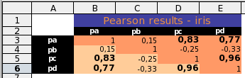
The procedure returns a table of correlation coefficients
Example 19.2. Pearson procedure
 table 'sport_cars':

    name        weight      speed    cost
    'skoda'      1200        260    10.000
    'renault'    1360        280    10.500
    'opel'       900         240    8.200
    'VW'         1400        280    12.00
    'Fiat'       1450        260    7.800
    'Alfa Romeo' 1300        280    11.000

result = pearson('sport_cars',[ 'weight', 'speed','cost'],sort = 0,silent=1)

strFormat = '%-10s%10s%10s%10s'
print strFormat % ('','weight','speed','cost')
strFormat = '%-10s%10.2f%10.2f%10.2f'
print strFormat % ('weight',1,result['weight']['speed'],result['weight']['cost'])
print strFormat % ('speed',result['speed']['weight'],1,result['speed']['cost'])
print strFormat % ('cost',result['cost']['weight'],result['cost']['speed'],1)
Output:
              weight     speed      cost
weight          1.00      0.76      0.37
speed           0.76      1.00      0.82
cost            0.37      0.82      1.00
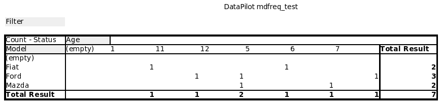
The mdfreq procedure is a powerful tool for cross tabulation. It uses OpenOffice DataPilot or MS Office PivotTable functions to create a pivot table. First, the dataset specified by the inTable parameter is copied into a spreadsheet (there are some limitations with respect to row and column count. The number of rows can not exceed ca. 32000 rows (in OpenOffice 2.0 and MS Office this limit has been raised to over 65000). The column count can not exceed 256). If the dataset is too large to fit in a spreadsheet, it si possible to use tableSplit or sample procedures to make a snapshot of the data.
After the data is copied into the spreadsheet, the Data Pilot is created.
See the diagram below for the description of the major parts of the OpenOffice Data Pilot object.
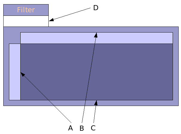
The marked parts are:
A - Cross table Rows
B - Cross table Columns
C - Cross table Data
D - Right Click at this area and select the "Start..." command to change the default Data Pilot settings
The MS Office pivotTable look similar, but part D, is replaced with an easy to use pivotTable manager.

MS Office 2003 and later versions have an interesting feature - data drill. By double clicking on a value in the generated table it is possible to see the source data value set used for counting the particular result.
By default Data Pilot is created using the first three categorical attributes from the dataset. The datapilot configuration can also be specified manually. If the table has less than three categorical values, it is possible to force mdfreq to treat numerical attributes as categorical using the categorical.
Syntax
mdfreq(alias.intable, categorical = [column_name, column_name, ... ], drop = [ column_name, column_name, ... ] )
intable - the name of the input table
categorical - list of attributes that should be treated as categorical
drop - list of attributes that should not be used in the Data Pilot
Example 19.3. The mdfreq procedure
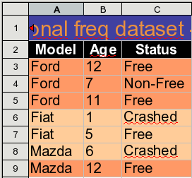
table 'mdfreq_test':
    Model     Age    Status
    'Ford'    12     'Free'
    'Ford'    7      'Non-Free'
    'Ford'    11     'Free'
    'Fiat'    1      'Crashed'
    'Fiat'    5      'Free'
    'Mazda'   6      'Crashed'
    'Mazda'   12     'Free'

mdfreq('mdfreq_test', categorical=['Age'])
Output:
*****Script 'mdfreq_docscript' finished after 2s. *****
The code above yields following spreadsheet