When the objective function and the constrains are defined, and the
optimization algorithm is chosen, then we are ready to solve the
optimization problem. One should define an Optimizer object, which has the
following parameters: the objective function, the optimization method, and
the constraints. Next one should apply the method optimize to this object.
The result of the method optimize is a point (vector) for which the
minimum is (or should be according to the algorithm) attained. During
optimization algorithm is able to generate some interesting information
about initial, transitive and final states what allows to evaluate the
converging process. Two
possible warnings in output: Step does not satisfy sufficient decrease
condition for the Newton, BCNewton, QuasiNewton, BCQusiNewton, FDNewton and
BCFDNewton methods and Mu is too small to continue for the Barrier methods.
The first type of warning occurs, for example, when the starting point is out of interval, on
which the objective function is minimized. The second type of warning informs that the
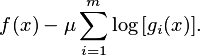
algorithm stopped because the barier parametr  was too small:
Example 18.8. Solving the optimization problem
from biz.sc.math.opt import *
from biz.sc.math.opt.alg import *
from biz.sc.math.opt.nlf import *
from biz.sc.math.opt.constraint import *

from java.util import ArrayList
from java.lang import System

from biz.sc.math.opt.nlf import *

class TestFunction(AbstractNLF):
    def __init__(self, dim, type):
        AbstractNLF.__init__(self, dim, type)
        print "Function dimension : ", dim
        print "Function type : ", type

    def evaluate(self, x, fx, gx, Hx):
        "@sig void evaluate(double[] x, double[] fx, double[] gx, double[][] Hx)"

        if (fx != None):
            fx[0] = x[0]*x[0]+x[1]*x[1]-2*x[1]

        if (gx != None):
            gx[0] = 2*x[0]
            gx[1] = 2*x[1]-2

        if (Hx != None):
            Hx[0][0] = Hx[1][1] = 2
            Hx[0][1] = Hx[1][0] = 0


constr = ArrayList()

bounds = BoundConstraint([1, .5],[2,1])

constr.add(bounds)

optMethod = BCNewtonMethod()

f = TestFunction(2, NLF.NLF2)
f.setInitVector([1.3,0.6])

opt = Optimizer(f, optMethod, constr)
opt.setMinimize();
opt.setOutput(sys.stdout, FALSE) # optimization information on standard output, false means without debug data

res = opt.optimize()

print res
Output:
Function dimension :  2
Function type :  2
**********************************************************
OPT++ version 2.1
Job run at Tue Sep 19 15:04:22 2006

**********************************************************
readOptInput: No opt.input file found
readOptInput: default values will be used


=========  Initial state  ===========


    i	    xc 		 grad 		 fcn_accrcy
     1         1.3	         2.6	    2.22e-16
     2         0.6	        -0.8	    2.22e-16
Function Value     =         0.85
Norm of gradient   =         2.72


==============================================


                Bound constrained Newton Method with Line Search

  Iter      F(x)       ||grad||     ||step||      f/g

    0         0.85         2.72
    1      0.09467        2.093       0.3139  N     2     2
OptBCNewton : variable added to working set : 1
OptBCNewton: Current working set
 ----- variable index:      1	1
     2            0            2       0.3077  N     3     3
checkConvg: gnorm =            0  gtol =    6.055e-06
OptBCNewton : variable added to working set : 2
OptBCNewton : reduced_grad_norm = 0
OptBCNewton: Current working set
 ----- variable index:      1	1     2	1
 OptBCNewtonLike : convergence achieved.


=========  Final state  ===========

Optimization method       = Bound constrained Newton
Dimension of the problem  = 2
No. of bound constraints  = 2
Return code               = 4 (Gradient tolerance test passed)
No. iterations taken      = 2
No. function evaluations  = 3
No. gradient evaluations  = 3


==========  Tolerances  ===========

Machine Epsilon      = 2.22045e-16
Maximum Step         = 1000
Minimum Step         = 1.49012e-08
Maximum Iter         = 100
Maximum Backtracks   = 5
Maximum Fcn Eval     = 1000
Step Tolerance       = 1.49012e-08
Function Tolerance   = 1.49012e-08
Constraint Tolerance = 1.49012e-08
Gradient Tolerance   = 6.05545e-06
LineSearch Tolerance = 0.0001


=========  Final state  ===========


    i	    xc 		 grad 		 fcn_accrcy
     1           1	           2	    2.22e-16
     2           1	           0	    2.22e-16
Function Value     =            0
Norm of gradient   =            2


==============================================

array([1.0, 1.0], double)
Note
It is recommended to use the setOutput(System.out, FALSE) method from the Optimizer class to print all the settings of the algorithm and the optimization process on the console.
When a product of a number of functions is minimized (e.g. the Likelihood function) it is better to minimize the logarithm of the object function, as the logarithm has a minimum in the same point as object function.
For methods that use constraints (all BC methods) the starting point has to be in the interval on which the objective function is minimized.